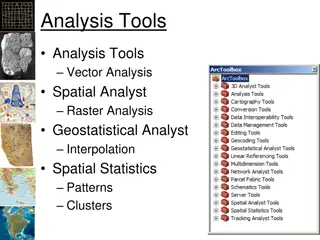
Spatial Interpolation with IDW Method
Spatial interpolation using the Inverse Distance Weighting (IDW) method is a technique to estimate unknown values between known data points. IDW determines cell values by giving greater weight to nearby points, creating an inverse relation between weighting and distance. This method works well for spatially auto-correlated features like elevation, property value, crime levels, and precipitation. IDW interpolation does not assume data trends but requires evenly spaced sample points. Learn how to perform IDW interpolation and control parameters to create accurate interpolated surfaces.

Download Presentation

Please find below an Image/Link to download the presentation.
The content on the website is provided AS IS for your information and personal use only. It may not be sold, licensed, or shared on other websites without obtaining consent from the author.If you encounter any issues during the download, it is possible that the publisher has removed the file from their server.
You are allowed to download the files provided on this website for personal or commercial use, subject to the condition that they are used lawfully. All files are the property of their respective owners.
The content on the website is provided AS IS for your information and personal use only. It may not be sold, licensed, or shared on other websites without obtaining consent from the author.
E N D
Presentation Transcript
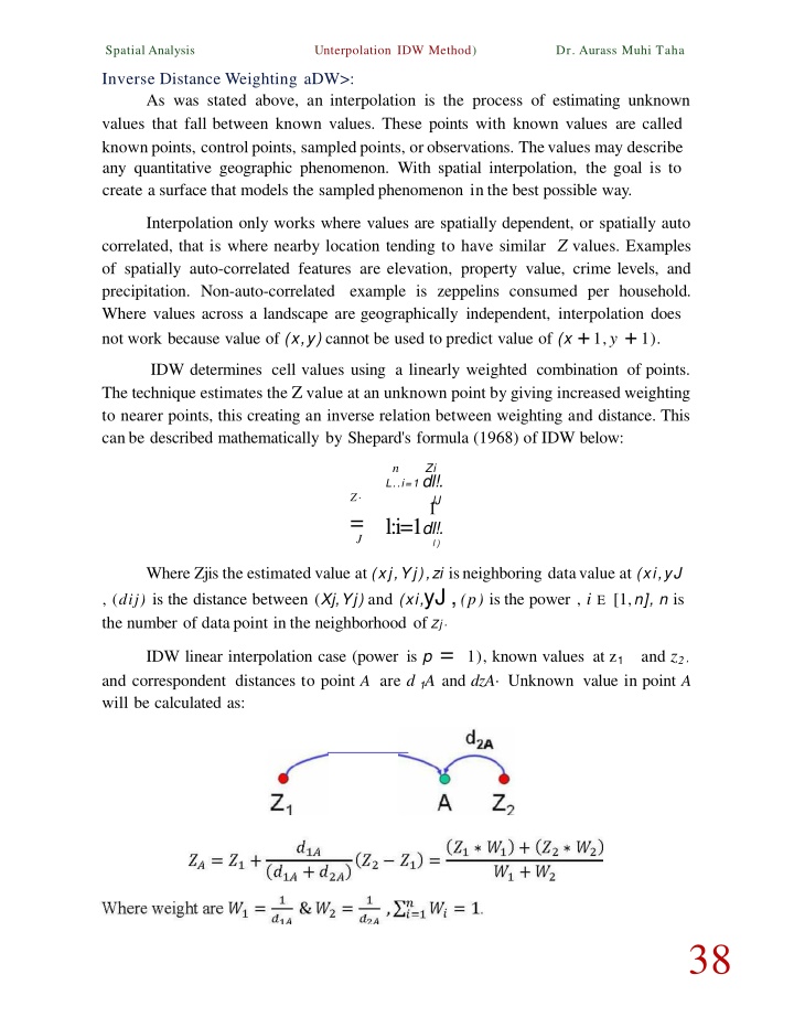
Spatial Analysis Unterpolation IDW Method) Dr. Aurass Muhi Taha Inverse Distance Weighting aDW>: As was stated above, an interpolation is the process of estimating unknown values that fall between known values. These points with known values are called known points, controlpoints, sampledpoints, orobservations. Thevalues may describe any quantitative geographic phenomenon. With spatial interpolation, the goal is to create a surface that models the sampled phenomenon in the best possible way. Interpolation only works where values are spatially dependent, or spatially auto correlated, that is where nearby location tending to have similar Z values. Examples of spatially auto-correlated features are elevation, property value, crime levels, and precipitation. Non-auto-correlated example is zeppelins consumed per household. Where values across a landscape are geographically independent, interpolation does not work because value of (x,y) cannot be used to predict value of (x +1,y + 1). IDW determines cell values using a linearly weighted combination of points. The technique estimates the Z value at an unknown point by giving increased weighting to nearer points, this creating an inverse relation between weighting and distance. This canbe described mathematically by Shepard's formula (1968) of IDW below: n Zi L..i=1 dl!. Z = J lJ1 l:i=1dl!. l ) Where Zjis the estimated value at (xj,Yj),zi isneighboring datavalue at (xi,yJ , (dij) is the distance between (Xj,Yj) and (xi,yJ , (p) is the power , i E [1,n], n is the number of datapoint in the neighborhood of Zj IDW linear interpolation case (power is p = 1), known values at z1 and correspondent distances to point A are d1A and dzA Unknown value in point A will be calculated as: and z2, 38
Spatial Analysis Unterpolation IDW Method) Dr. Aurass Muhi Taha IDW Features: IDW description of an interpolated surface. There are no assumptions required of the data, but there is no assessment of prediction errors. IDW works best for dense, evenly spaced sample points. It does not consider trends in the data and cannot make estimates above the maximum or below the minimum sample values. The IDW model parameters: a good preliminary can provide The characteristics of the interpolated surface in IDW interpolation can be controlled by the following parameters: a)By value of the power function. b)By the neighborhood search strategy that is limiting the number of input points that can be used in calculating the value of each interpolated point. Limit of control points canbe definedby: 1.A number of closest sample points used. 2. A search radius used for searchneighborhood. 3. A shape of searchneighborhood. 4. A combination of above strategies. Creating a map using IDW: IDW assumes that the surface is being driven by local variation. It works better if sample points are evenly distributed throughout the area and if they are not clustered. The important parameters are the search neighborhood specifications, the power parameter .p., and the anisotropy (see Chapter 3, .The principles of geostatistical analysis.) factor if one exists. Steps: 1. Click onthe point layer onwhich to perform IDW in theArcMap table of contents. 2. Startthe Geostatistical Analyst. 3. Click theAttribute dropdown menu and click the attribute onwhich to perform IDW in the Choose Input Data andMethod dialog box. 4. Click the Inverse Distance Weighting method. 5. Click Next. 6. Specify the desired parameters inthe IDW SetParameters dialog box andclick next. 7. Examine the results onthe Cross Validation dialog box and click Finish. 8. Click onthe Output Layer Information dialog box and click OK. 39
Spatial Analysis Unterpolation IDW Method) Dr. Aurass Muhi Taha ,. - lnw't Sd bbn Gtoproccs.Mng C om :t " Http > "" <t,. 0 M [!;JG;Ip;i!iiiO ) i , I - ''"'""''""'" 3 ! } IJJ , . > : GPS II. CIEHi10 .tl. ft 6 .:.. :. () : : : . . ill It ; . . _..-a . l , '"' 3 "' I Ji, l s lll.,.,.... on:.t100 b. G q,., t 9,.. .. IQ : I;_,). r- ,. r - - - - - - - - - - - - - - - - - - - - - - -- - - - - - - - - - - - - -- - - - - - - -- - - - - - - - - - - - . R.s uClc.nup CdStl t10tt l&tOf " labl\1!:Of (OI'IttnlJ Elllv 8 . , . . . ,1i! IllY .iJ Locals-dl . .. .. I ermkllstic methods_ j 8 Dataset Sou"ceOa aSet !DIY IS A R w I GlobalPolyncmallnt!rpolalion RacialBasisfu'lcbOnS LocalPolynomialinterpolation 8 Geostatistic:al methods KrigingICoKriQi1o Arelll lntl!f'PC)Iation S..yesoanKriging 8 Interpolation with baniers Kern<Smoothino DiffusiooKemoj Inverse Distance Weighting D i s t a n c e Weighting (lOW)isaquid<det.!!rmi"isticlntl!f'PC)Iator !hatiseJ<aCt.Thereaceveryfewdeocisionsto makrreo.Ydno1110d<!parameters. It canbeaooodway to a ftst lookatanlntl!f'PC)Iated - However, the-eisnoassessment of P acOU>ddatalocations.Thl!reacenoassulllbOnS r e d ofthedata. ef!'OI'S, and!DIYcanproducl! W s eyes t 40
SpatialAnalysis Unterpolation IDW Method) Dr. Aurass Muhi Taha 8 GenooralProl><'rti<os Power 8 arch Heighbortlood I ' I P " ' Maxirunneighbors Mlninunneighbors S torl'fP"' &;. 2 Stanc!Nd lS 10 0 1S tor Major se'nilllds notsetM Mi " 8 l e n d Value y 0.3l37036 0.3137036 JOS 44.528'18 32.35851 s . 8 Weights (15 neighbors) <rnor.,> GoonooralProl><'rti<os Dis!anreWelg\llng {lOW)ISa Q t O d <df!tenrri;tic Interpolator lhatis IO>Ga<t.Thereare-my l'ewdo!dsions to . . <Bad< 8 Gene. ral Properties Powe- 8 Sea . rch Neighborhood . .. 2 Smooth 0.2 lo 0.3137036 0.3137036 MajOr sellalOS Minor semoalds 8 Predicted Value X y 44.528'18 32.35851 0 8 Weights (61neighbors) N eighborhood type Standard opllonwl assignweghts based oncistance from the target locallon. Smooth opllonadjusts thew . <moro o> N<oxt > <Back 41
SpatialAnalysis Unterpolation IDW Method) Dr. Aurass Muhi Taha . ' : ": . . , .. . .. ,., Sau-ce ID Included . . . - . . . . . , MeaSU'ed Predicted Error , , , \ ( (" ,. Predicted 101 1062 Y es Yes Yes Yes Yes Y es Yes Yes Yes Yes Yes Yes Yes Y es Y es Yes Yes Yes Y es Y es Y es Y es Yes Yes Yes Yes Yt>< 0 1.12 3.6 5.83 6.65 8.38 10.04 1.26 4.21 6.47 7.15 9.18 2.92 6.33 7.29 7.71 10.26 1.61 5.97 4.4 7.94 10.62 9.7 8.73 8.17 4.1 8 3.53 1.17 1.676... 3.3'18. . '1.986... '1.219... '1.858... 3.973... 2.152... 0.968... 0.99'1... 3.921... 3.284... 2.'185... 2.901... 3.853... 2.842... 3.001.. 3.393... -1.1'11... '1.261... 3.'i04... 2.420... 2.'101... 7.298778438796595 3.0'i0... 5.6898145'10087966 2.866... 5 .30301'18036964935 1.8'12... -2.337001'i0'1823353'1 1.166... 2.363750038208075'1 ,.I'VI... 1.011071 QlRM 701 o.556779'1948690994 .0.25172021442443215 -().8'136103778031319 2.'1309569217812097 3.521578350225079 .066372355258442 0.8920367478113749 3.2'113511022730317 5.'17559'1969881519 3.2288950076820107 5.895'177327860762 .0.'13'127023579552'16 3.428226814'1876107 3.'1369014969233143 -4.867301995677833 .7.258244268882227 1.78369682334450 1 6 1.8281299779'121927 -o.138'1763654007'1n -4.535499450809564 -a.199102357596813 0 . 9-l.! 2 3 'I 5 6 7 8 9 10 11 12 13 14 15 16 17 18 19 20 21 22 23 24 25 ]F. < 0.826 0.708 . . .:.. 0.591 OAn a / I .. / . / . ?. t .. . ... 0.354 1 0.236 1 o.11s / 1.062 0.796 Measured 10 1 0 0.266 0531 Precicted , Erro.-, IR ession Mction Pred'ICtion Errors lo.09016000939n626 ...1 nofn .0.3428562 3.690864 Mean Root an-Square El<portReslJtTable v > <Bedc Arist1 Gc9po""aoW19 c:""-" w ,-..., filii. View Ci6 1i1 - - Hdp < ! : > !1 1. n It 0 C ! 3 ,:.;. ft o! :J ,O., ; f ; b ::::Jt U l a i Y J.GOS /i> '"' ., vj G l ! M ii;;lliii H!:J>.., If.>'ow t'il'"' o..,.,...., . r-j----- ::::J:-1 -Gco ISt t t t C ): :: + - I .o., ..t..... -1,.1 ::::J n.., ::::J --- --..h G<OI .,_., . 1 - : : ; _. 0 0 - f ; Rauet Clur!up Cd Sd tiott ,. -- fxr------ ------------ f X -......, . C o n tOUR O I.072Q}M9 1.onolle9 Z.IOIC6109 a L I t - 1.0917296! 3.091n963 4.042ft11JJ 4.0ol261tll- S.OW7 7 s.oll27591 6.o6lJQJ17 6.0QJO-J77-7.1J.&).Il.46 7.UollU4&-12!010l.U 8.2i0102-'1- U1U699S 9:41B699S- hl62 li!I I O W ! 0 ; 1 - !iW ..<T..., o -"'9' D A 42