Statistical Analysis for Detecting Benzene Concentration - Methods & Confidence Intervals
Exploring statistical methods for detecting benzene concentrations in blood samples, calculating critical levels, minimum detectable values, confidence intervals, regression analysis for zinc measurements, and assessing regression assumptions.
Download Presentation

Please find below an Image/Link to download the presentation.
The content on the website is provided AS IS for your information and personal use only. It may not be sold, licensed, or shared on other websites without obtaining consent from the author.If you encounter any issues during the download, it is possible that the publisher has removed the file from their server.
You are allowed to download the files provided on this website for personal or commercial use, subject to the condition that they are used lawfully. All files are the property of their respective owners.
The content on the website is provided AS IS for your information and personal use only. It may not be sold, licensed, or shared on other websites without obtaining consent from the author.
E N D
Presentation Transcript
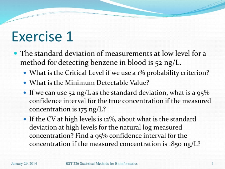
Exercise 1 The standard deviation of measurements at low level for a method for detecting benzene in blood is 52 ng/L. What is the Critical Level if we use a 1% probability criterion? What is the Minimum Detectable Value? If we can use 52 ng/L as the standard deviation, what is a 95% confidence interval for the true concentration if the measured concentration is 175 ng/L? If the CV at high levels is 12%, about what is the standard deviation at high levels for the natural log measured concentration? Find a 95% confidence interval for the concentration if the measured concentration is 1850 ng/L? January 29, 2014 BST 226 Statistical Methods for Bioinformatics 1
= = = 52 ng/L 0.01 0.01 + + = + = CL = 0 MDV= 0 95% CI (52)(2.326) 121 ng/L ( ) (52)(2.326 2.326) 175 (52)(1.960) 175 102 [73,277] ng/L If the high level CV is about 12%, then the natural log measurement has 0.12 ln(1850) (0.12)(1.960) 7.523 0.235 [7.288,7.758] in ln units =[1462,2341] ng/L ( ) ( ) z z = + = 242 ng/L z = = = of the = = = = 95% CI January 29, 2014 BST 226 Statistical Methods for Bioinformatics 2
Exercise 2 Download data on measurement of zinc in water by ICP/MS ( Zinc.csv ). Use read.csv() to load. Conduct a regression analysis in which you predict peak area from concentration Which of the usual regression assumptions appears to be satisfied and which do not? What would the estimated concentration be if the peak area of a new sample was 1850? From the blanks part of the data, how big should a result be to indicate the presence of zinc with some degree of certainty? Try using weighted least squares for a better estimate of the calibration curve. Does it seem to make a difference? January 29, 2014 BST 226 Statistical Methods for Bioinformatics 3
zinc <- read.csv("zinc.csv") > names(zinc) [1] "Concentration" "Peak.Area" > zinc.lm <- lm(Peak.Area ~ Concentration,data=zinc) > summary(zinc.lm) Call: lm(formula = Peak.Area ~ Concentration, data = zinc) Residuals: Min 1Q Median 3Q Max -11242.22 -82.01 333.28 485.89 9353.28 Coefficients: Estimate Std. Error t value Pr(>|t|) (Intercept) 104.5429 267.1370 0.391 0.696 Concentration 7.2080 0.0307 234.769 <2e-16 *** --- Signif. codes: 0 *** 0.001 ** 0.01 * 0.05 . 0.1 1 Residual standard error: 2201 on 89 degrees of freedom Multiple R-squared: 0.9984, Adjusted R-squared: 0.9984 F-statistic: 5.512e+04 on 1 and 89 DF, p-value: < 2.2e-16 > plot(zinc$Concentration,zinc$Peak.Area) > abline(coef(zinc.lm)) > plot(fitted(zinc.lm),resid(zinc.lm)) > (1850-104.5429)/7.2080 [1] 242.1555 January 29, 2014 BST 226 Statistical Methods for Bioinformatics 4
January 29, 2014 BST 226 Statistical Methods for Bioinformatics 5
January 29, 2014 BST 226 Statistical Methods for Bioinformatics 6
> zinc[zinc$Concentration==0,] Concentration Peak.Area 1 0 115 2 0 631 3 0 508 4 0 317 5 0 220 6 0 93 7 0 99 8 0 135 The CL in peak area terms is 742, with zero concentration indicated at 265. The CL in ppt is (742 104.5429)/7.2080 = 88 ppt. The MDV is 176 ppt. No samples for true concentrations of 0, 10, or 20 had peak areas above the CL. For the samples at 100ppt or above, all had peak areas above the CL of 742. > mean(zinc[zinc$Concentration==0,2]) [1] 264.75 > sd(zinc[zinc$Concentration==0,2]) [1] 205.0343 264.75+2.326*205.3 [1] 742.2778 January 29, 2014 BST 226 Statistical Methods for Bioinformatics 7
> summary(lm(Peak.Area ~ Concentration,data=zinc)) Coefficients: Estimate Std. Error t value Pr(>|t|) (Intercept) 104.5429 267.1370 0.391 0.696 Concentration 7.2080 0.0307 234.769 <2e-16 *** > vars <- tapply(zinc$Peak,zinc$Conc,var) 0 10 20 100 200 500 1000 4.203907e+04 1.714762e+02 7.869524e+02 1.438745e+04 1.431810e+03 8.074238e+03 5.365478e+04 2000 5000 10000 25000 4.098095e+04 1.849742e+06 1.358443e+07 2.835566e+07 > concs <- unique(zinc$Conc) > concnums <- table(zinc$Conc) 0 10 20 100 200 500 1000 2000 5000 10000 25000 8 7 7 11 7 7 9 7 9 10 9 January 29, 2014 BST 226 Statistical Methods for Bioinformatics 8
> summary(lm(Peak.Area ~ Concentration,data=zinc)) Coefficients: Estimate Std. Error t value Pr(>|t|) (Intercept) 104.5429 267.1370 0.391 0.696 Concentration 7.2080 0.0307 234.769 <2e-16 *** > vars <- tapply(zinc$Peak,zinc$Conc,var) > concs <- unique(zinc$Conc) > concnums <- table(zinc$Conc) > concs2 <- concs^2 > var.lm <- lm(vars ~ concs2) > rbind(vars,predict(var.lm)) 0 10 20 100 200 500 1000 2000 5000 vars 42039.07 171.4762 786.9524 14387.45 1431.81 8074.238 53654.78 40980.95 1849742 829839.07 829843.6834 829857.5149 830300.12 831683.27 841365.323 875944.07 1014259.07 1982464 > wt1 <- 1/rep(vars,concnums) > wt2 <- 1/rep(predict(var.lm),concnums) > summary(lm(Peak.Area ~ Concentration,data=zinc,weights=wt1)) Coefficients: Estimate Std. Error t value Pr(>|t|) (Intercept) 333.9925 18.9250 17.65 <2e-16 *** Concentration 7.4117 0.1103 67.21 <2e-16 *** > summary(lm(Peak.Area ~ Concentration,data=zinc,weights=wt2)) Coefficients: Estimate Std. Error t value Pr(>|t|) (Intercept) 433.20668 91.07209 4.757 7.55e-06 *** Concentration 7.06868 0.03555 198.864 < 2e-16 *** January 29, 2014 BST 226 Statistical Methods for Bioinformatics 9
Exercise 3 The file hiv.csv contains data on an HIV PCR assay calibration. These are dilutions of ten samples at 15 copy numbers from 25 to 20,000,000. In theory, the Ct value (Target in the data set) should be linear in log copy number. Fit the calibration line and look at plots to examine the assumptions of linear regression. What is the estimated copy number for an unknown if Ct = 25? The column QS is the Ct value for an in-tube standard. Consider calibrating Ct(Target) Ct(Standard) instead. Does this work better or not? What is a good criterion? January 29, 2014 BST 226 Statistical Methods for Bioinformatics 10
> hiv.lm <- lm(Target ~ log(Nominal),data=hiv) > summary(hiv.lm) Call: lm(formula = Target ~ log(Nominal), data = hiv) Residuals: Min 1Q Median 3Q Max -9.7150 -0.4416 -0.1037 0.3057 8.6227 Coefficients: Estimate Std. Error t value Pr(>|t|) (Intercept) 38.930434 0.061413 633.9 <2e-16 *** log(Nominal) -1.385832 0.005831 -237.7 <2e-16 *** --- Signif. codes: 0 *** 0.001 ** 0.01 * 0.05 . 0.1 1 Residual standard error: 0.8828 on 878 degrees of freedom Multiple R-squared: 0.9847, Adjusted R-squared: 0.9847 F-statistic: 5.649e+04 on 1 and 878 DF, p-value: < 2.2e-16 January 29, 2014 BST 226 Statistical Methods for Bioinformatics 11
> anova(hiv.lm) Analysis of Variance Table Response: Target Df Sum Sq Mean Sq F value Pr(>F) log(Nominal) 1 44026 44026 56489 < 2.2e-16 *** Residuals 878 684 1 --- Signif. codes: 0 *** 0.001 ** 0.01 * 0.05 . 0.1 1 January 29, 2014 BST 226 Statistical Methods for Bioinformatics 12
January 29, 2014 BST 226 Statistical Methods for Bioinformatics 13
Calibration Results Variance is not constant, being higher at higher Ct levels. Adding the standard helps unless copy number is very high (more than 1 million) Using the Target ~ regression, a Ct value of 25 corresponds to a log copy number of (25 38.93)/( 1.386) = 10.05 Copy number = exp(10.05) = 23,167 January 29, 2014 BST 226 Statistical Methods for Bioinformatics 14
SD ratio Target ~ vs Target QS ~ Use of standard is better when copy number > 100 and less than 5 million January 29, 2014 BST 226 Statistical Methods for Bioinformatics 15
Exercise 4 The file AD-Luminex.csv contains Luminex protein assays for 124 proteins on 104 patients who are either AD (Alzheimer's Disease, OD (other dementia) or NDC (non-demented controls). See if the measured levels of ApoE are associated with diagnosis. See if the measured levels of IL.1beta are associated with diagnosis. January 29, 2014 BST 226 Statistical Methods for Bioinformatics 16
> ad.data <- read.csv("AD-Luminex.csv") > anova(lm(ApoE ~ Diagnosis,data=ad.data)) Analysis of Variance Table Response: ApoE Df Sum Sq Mean Sq F value Pr(>F) Diagnosis 2 877.9 438.93 3.3662 0.03844 * Residuals 101 13169.8 130.39 --- Signif. codes: 0 *** 0.001 ** 0.01 * 0.05 . 0.1 1 > anova(lm(log(ApoE) ~ Diagnosis,data=ad.data)) Analysis of Variance Table Response: log(ApoE) Df Sum Sq Mean Sq F value Pr(>F) Diagnosis 2 3.1377 1.56885 6.1503 0.003016 ** Residuals 101 25.7636 0.25508 --- Signif. codes: 0 *** 0.001 ** 0.01 * 0.05 . 0.1 1 January 29, 2014 BST 226 Statistical Methods for Bioinformatics 17
> anova(lm(IL.1beta ~ Diagnosis,data=ad.data)) Analysis of Variance Table Response: IL.1beta Df Sum Sq Mean Sq F value Pr(>F) Diagnosis 2 15.20 7.5992 1.0918 0.3395 Residuals 101 702.97 6.9601 > anova(lm(log(IL.1beta) ~ Diagnosis,data=ad.data)) Analysis of Variance Table Response: log(IL.1beta) Df Sum Sq Mean Sq F value Pr(>F) Diagnosis 2 1.861 0.93033 2.5717 0.0814 . Residuals 101 36.538 0.36176 --- Signif. codes: 0 *** 0.001 ** 0.01 * 0.05 . 0.1 1 January 29, 2014 BST 226 Statistical Methods for Bioinformatics 18
January 29, 2014 BST 226 Statistical Methods for Bioinformatics 19
January 29, 2014 BST 226 Statistical Methods for Bioinformatics 20
January 29, 2014 BST 226 Statistical Methods for Bioinformatics 21
January 29, 2014 BST 226 Statistical Methods for Bioinformatics 22
