Statistical Analysis of Laboratory Data: Learning Methods and Distance Measures
Explore supervised learning with logistic regression and Fisher's LDA, unsupervised learning methods, cluster analysis, and the significance of distance measures in clustering methods. Understand the concept of true distance metrics like Euclidean distance for effective data analysis.

Download Presentation

Please find below an Image/Link to download the presentation.
The content on the website is provided AS IS for your information and personal use only. It may not be sold, licensed, or shared on other websites without obtaining consent from the author. If you encounter any issues during the download, it is possible that the publisher has removed the file from their server.
You are allowed to download the files provided on this website for personal or commercial use, subject to the condition that they are used lawfully. All files are the property of their respective owners.
The content on the website is provided AS IS for your information and personal use only. It may not be sold, licensed, or shared on other websites without obtaining consent from the author.
E N D
Presentation Transcript
SPH 247 Statistical Analysis of Laboratory Data May 26, 2015 SPH 247 Statistical Analysis of Laboratory Data 1
Supervised and Unsupervised Learning Logistic regression and Fisher s LDA and QDA are examples of supervised learning. This means that there is a training set which contains known classifications into groups that can be used to derive a classification rule. This can be then evaluated on a test set , or this can be done repeatedly using cross validation. May 26, 2015 SPH 247 Statistical Analysis of Laboratory Data 2
Unsupervised Learning Unsupervised learning means (in this instance) that we are trying to discover a division of objects into classes without any training set of known classes, without knowing in advance what the classes are, or even how many classes there are. It should not have to be said that this is a difficult task May 26, 2015 SPH 247 Statistical Analysis of Laboratory Data 3
Cluster Analysis Cluster analysis , or simply clustering is a collection of methods for unsupervised class discovery These methods are widely used for gene expression data, proteomics data, and other omics data types They are likely more widely used than they should be One can cluster subjects (types of cancer) or genes (to find pathways or co-regulation) or both at the same time. May 26, 2015 SPH 247 Statistical Analysis of Laboratory Data 4
Distance Measures It turns out that the most crucial decision to make in choosing a clustering method is defining what it means for two vectors to be close or far. There are other components to the choice, but these are all secondary Often the distance measure is implicit in the choice of method, but a wise decision maker knows what he/she is choosing. May 26, 2015 SPH 247 Statistical Analysis of Laboratory Data 5
A true distance, or metric, is a function defined on pairs of objects that satisfies a number of properties: D(x,y) = D(y,x) D(x,y) 0 D(x,y) = 0 x = y D(x,y) + D(y,z) D(x,z) (triangle inequality) The classic example of a metric is Euclidean distance. If x = (x1,x2, xp), and y=(y1,y2, yp) , are vectors, the Euclidean distance is [(x1-y1)2+ (xp-yp)2] May 26, 2015 SPH 247 Statistical Analysis of Laboratory Data 6
Euclidean Distance y = (y1,y2) D(x,y) |x2-y2| |x1-y1| x = (x1,x2) May 26, 2015 SPH 247 Statistical Analysis of Laboratory Data 7
Triangle Inequality x D(x,z) D(x,y) y D(y,z) z May 26, 2015 SPH 247 Statistical Analysis of Laboratory Data 8
Other Metrics The city block metric is the distance when only horizontal and vertical travel is allowed, as in walking in a city. It turns out to be |x1-y1|+ |xp-yp| instead of the Euclidean distance [(x1-y1)2+ (xp-yp)2] May 26, 2015 SPH 247 Statistical Analysis of Laboratory Data 9
Mahalanobis Distance Mahalanobis distance is a kind of weighted Euclidean distance It produces distance contours of the same shape as a data distribution It is often more appropriate than Euclidean distance when there are not too many variables May 26, 2015 SPH 247 Statistical Analysis of Laboratory Data 10
May 26, 2015 SPH 247 Statistical Analysis of Laboratory Data 11
May 26, 2015 SPH 247 Statistical Analysis of Laboratory Data 12
May 26, 2015 SPH 247 Statistical Analysis of Laboratory Data 13
Non-Metric Measures of Similarity A common measure of similarity used for microarray data is the (absolute) correlation. This rates two data vectors as similar if they move up and down together, without worrying about their absolute magnitudes This is not a metric, since if violates several of the required properties We could use 1 - | | as the distance May 26, 2015 SPH 247 Statistical Analysis of Laboratory Data 14
Agglomerative Hierarchical Clustering We start with all data items as individuals In step 1, we join the two closest individuals In each subsequent step, we join the two closest individuals or clusters This requires defining the distance between two groups as a number that can be compared to the distance between individuals We can use the R commands hclust or agnes May 26, 2015 SPH 247 Statistical Analysis of Laboratory Data 15
Group Distances Complete link clustering defines the distance between two groups as the maximum distance between any element of one group and any of the other Single link clustering defines the distance between two groups as the minimum distance between any element of one group and any of the other Average link clustering defines the distance between two groups as the mean distance between elements of one group and elements of the other May 26, 2015 SPH 247 Statistical Analysis of Laboratory Data 16
May 26, 2015 SPH 247 Statistical Analysis of Laboratory Data 17
> iris.d <- dist(iris[,1:4]) > iris.hc <- hclust(iris.d) > plot(iris.hc) > par(pin=c(10,5)) > par(cex=.8) > plot(iris.hc,labels=rep(c("S","C","I"),each=50), xlab="",sub="",ylab="",main="Iris Cluster Plot") > plot(hclust(dist(t(exprs(eset.lmg))))) > plot(hclust(as.dist(1-cor(exprs(eset.lmg))^2))) May 26, 2015 SPH 247 Statistical Analysis of Laboratory Data 18
May 26, 2015 SPH 247 Statistical Analysis of Laboratory Data 19
May 26, 2015 SPH 247 Statistical Analysis of Laboratory Data 20
May 26, 2015 SPH 247 Statistical Analysis of Laboratory Data 21
Divisive Clustering Divisive clustering begins with the whole data set as a cluster, and considers dividing it into k clusters. Usually this is done to optimize some criterion such as the ratio of the within cluster variation to the between cluster variation The choice of k is important May 26, 2015 SPH 247 Statistical Analysis of Laboratory Data 22
K-means is a widely used divisive algorithm (R command kmeans) Its major weakness is that it uses Euclidean distance Some other routines in R for divisive clustering include agnes and fanny in the cluster package (library(cluster)) May 26, 2015 SPH 247 Statistical Analysis of Laboratory Data 23
> iris.km <- kmeans(iris[,1:4],3) > plot(prcomp(iris[,1:4])$x,col=iris.km$cluster) > > table(iris.km$cluster,iris[,5]) setosa versicolor virginica 1 0 48 14 2 0 2 36 3 50 0 0 > May 26, 2015 SPH 247 Statistical Analysis of Laboratory Data 24
May 26, 2015 SPH 247 Statistical Analysis of Laboratory Data 25
> rice.km2 <- kmeans(t(exprs(eset.lmg)),2) > rice.km3 <- kmeans(t(exprs(eset.lmg)),3) > rice.km4 <- kmeans(t(exprs(eset.lmg)),4) > rice.km5 <- kmeans(t(exprs(eset.lmg)),5) > rice.km6 <- kmeans(t(exprs(eset.lmg)),6) May 26, 2015 SPH 247 Statistical Analysis of Laboratory Data 26
> table(rice.km2$cluster,group) group 0 1 2 3 4 5 1 0 0 2 2 0 0 2 2 2 0 0 2 2 > table(rice.km3$cluster,group) group 0 1 2 3 4 5 1 2 2 0 0 0 0 2 0 0 2 2 0 0 3 0 0 0 0 2 2 > table(rice.km4$cluster,group) group 0 1 2 3 4 5 1 0 0 0 0 2 2 2 0 0 2 2 0 0 3 1 0 0 0 0 0 4 1 2 0 0 0 0 > table(rice.km5$cluster,group) group 0 1 2 3 4 5 1 0 0 1 2 0 0 2 0 0 0 0 2 2 3 1 0 0 0 0 0 4 0 0 1 0 0 0 May 26, 2015 SPH 247 Statistical Analysis of Laboratory Data 27
> table(rice.km6$cluster,group) group 0 1 2 3 4 5 1 1 0 0 0 0 0 2 0 0 0 0 2 1 3 1 2 0 0 0 0 4 0 0 0 0 0 1 5 0 0 1 2 0 0 6 0 0 1 0 0 0 May 26, 2015 SPH 247 Statistical Analysis of Laboratory Data 28
Model-based clustering methods allow use of more flexible shape matrices. One such package is mclust, which needs to be downloaded from CRAN Functions in this package include EMclust (more flexible), Mclust (simpler to use) Other excellent software is EMMIX from Geoff McLachlan at the University of Queensland. May 26, 2015 SPH 247 Statistical Analysis of Laboratory Data 29
Models compared in mclust: univariateMixture A vector with the following components: "E": equal variance (one-dimensional) "V": variable variance (one-dimensional) multivariateMixture A vector with the following components: "EII": spherical, equal volume "VII": spherical, unequal volume "EEI": diagonal, equal volume and shape "VEI": diagonal, varying volume, equal shape "EVI": diagonal, equal volume, varying shape "VVI": diagonal, varying volume and shape "EEE": ellipsoidal, equal volume, shape, and orientation "EEV": ellipsoidal, equal volume and equal shape "VEV": ellipsoidal, equal shape "VVV": ellipsoidal, varying volume, shape, and orientation singleComponent A vector with the following components: "X": one-dimensional "XII": spherical "XXI": diagonal "XXX": ellipsoidal May 26, 2015 SPH 247 Statistical Analysis of Laboratory Data 30
> data(iris) > mc.obj <- Mclust(iris[,1:4]) > plot.Mclust(mc.obj,iris[1:4]) May 26, 2015 SPH 247 Statistical Analysis of Laboratory Data 31
-600 -800 -1000 -1200 BIC -1400 -1600 EII VII EEI VEI EVI VVI EEE EEV VEV VVV -1800 2 4 6 8 number of components May 26, 2015 SPH 247 Statistical Analysis of Laboratory Data 32
2.0 2.5 3.0 3.5 4.0 0.5 1.0 1.5 2.0 2.5 7.5 6.5 Sepal.Length 5.5 4.5 4.0 3.5 Sepal.Width 3.0 2.5 2.0 7 6 5 Petal.Length 4 3 2 1 2.5 2.0 1.5 Petal.Width 1.0 0.5 4.5 5.5 6.5 7.5 1 2 3 4 5 6 7 May 26, 2015 SPH 247 Statistical Analysis of Laboratory Data 33
1,2 Coordinate Projection showing Classification 4.0 3.5 Sepal.Width 3.0 2.5 2.0 4.5 5.0 5.5 6.0 6.5 7.0 7.5 8.0 Sepal.Length May 26, 2015 SPH 247 Statistical Analysis of Laboratory Data 34
1,2 Coordinate Projection showing Uncertainty 4.0 3.5 Sepal.Width 3.0 2.5 2.0 4.5 5.0 5.5 6.0 6.5 7.0 7.5 8.0 Sepal.Length May 26, 2015 SPH 247 Statistical Analysis of Laboratory Data 35
> names(mc.obj) [1] "modelName" "n" "d" "G" [5] "BIC" "bic" "loglik" "parameters" [9] "z" "classification" "uncertainty" > mc.obj$bic [1] -561.7285 > mc.obj$BIC EII VII EEI VEI EVI VVI EEE 1 -1804.0854 -1804.0854 -1522.1202 -1522.1202 -1522.1202 -1522.1202 -829.9782 2 -1123.4115 -1012.2352 -1042.9680 -956.2823 -1007.3082 -857.5515 -688.0972 3 -878.7651 -853.8145 -813.0506 -779.1565 -797.8356 -744.6356 -632.9658 4 -784.3102 -783.8267 -735.4820 -716.5253 -732.4576 -705.0688 -591.4097 5 -734.3865 -746.9931 -694.3922 -703.0523 -695.6736 -700.9100 -604.9299 6 -715.7148 -705.7813 -693.8005 -675.5832 -722.1517 -696.9024 -621.8177 7 -712.1014 -708.7210 -671.6757 -666.8672 -704.1649 -703.9925 -617.6212 8 -686.0967 -707.2610 -661.0846-657.2447 -703.6602 -702.1138 -622.4221 9 -694.5242 -700.0220 -678.5986 -671.8247 -737.3109 -727.6346 -638.2076 EEV VEV VVV 1 -829.9782 -829.9782 -829.9782 2 -644.5997 -561.7285-574.0178 3 -610.0853 -562.5514 -580.8399 4 -646.0011 -603.9266 -628.9650 5 -621.6906 -635.2087 -683.8206 6 -669.7188 -681.3062 -711.5726 7 -711.3150 -715.2100 -728.5508 8 -750.1897 -724.1750 -801.7295 9 -799.6408 -810.1318 -835.9095 May 26, 2015 SPH 247 Statistical Analysis of Laboratory Data 36
Clustering Genes Clustering genes is relatively easy, in the sense that we treat an experiment with 60 arrays and 9,000 genes as if the sample size were 9,000 and the dimension 60 Extreme care should be taken in selection of the explicit or implicit distance function, so that it corresponds to the biological intent This is used to find similar genes, identify putative co-regulation, and reduce dimension by replacing a group of genes by the average May 26, 2015 SPH 247 Statistical Analysis of Laboratory Data 37
Clustering Samples This is much more difficult, since we are using the sample size of 60 and dimension of 9,000 K-means and hierarchical clustering can work here Model-based clustering requires substantial dimension reduction either by gene selection or use of PCA or similar methods May 26, 2015 SPH 247 Statistical Analysis of Laboratory Data 38
Heatmaps A heatmap displays a clustering of the samples and the genes using a false color plot. It may or may not be useful in a given situation. > heatmap(exprs(eset.lmg)) > Library(RColorBrewer) > heatmap(exprs(eset.lmg),col=brewer.pal(7,"RdYlGn")) May 26, 2015 SPH 247 Statistical Analysis of Laboratory Data 39
May 26, 2015 SPH 247 Statistical Analysis of Laboratory Data 40
May 26, 2015 SPH 247 Statistical Analysis of Laboratory Data 41
Cautionary Notes Cluster analysis is by far the most difficult type of analysis one can perform. Much about how to do cluster analysis is still unknown. There are many choices that need to be made about distance functions and clustering methods and no clear rule for making the choices May 26, 2015 SPH 247 Statistical Analysis of Laboratory Data 42
Hierarchical clustering is really most appropriate when there is a true hierarchy thought to exist in the data; an example would be phylogenetic studies. The ordering of observations in a hierarchical clustering is often interpreted. However, for a given hierarchical clustering of, say, 60 cases, there are 5 1017 possible orderings, all of which are equally valid. With 9,000 genes, the number of orderings in unimaginably huge, approximate 102700 May 26, 2015 SPH 247 Statistical Analysis of Laboratory Data 43
Exercises In the ISwR data set alkfos, cluster the data based on the 7 measurements using hclust(), kmeans(), and Mclust(). Compare the 2-group clustering with the placebo/Tamoxifen classification. May 26, 2015 SPH 247 Statistical Analysis of Laboratory Data 44


")


")

),2)")
")
")


")


")