Statistical Analysis Techniques in Biological Data Processing

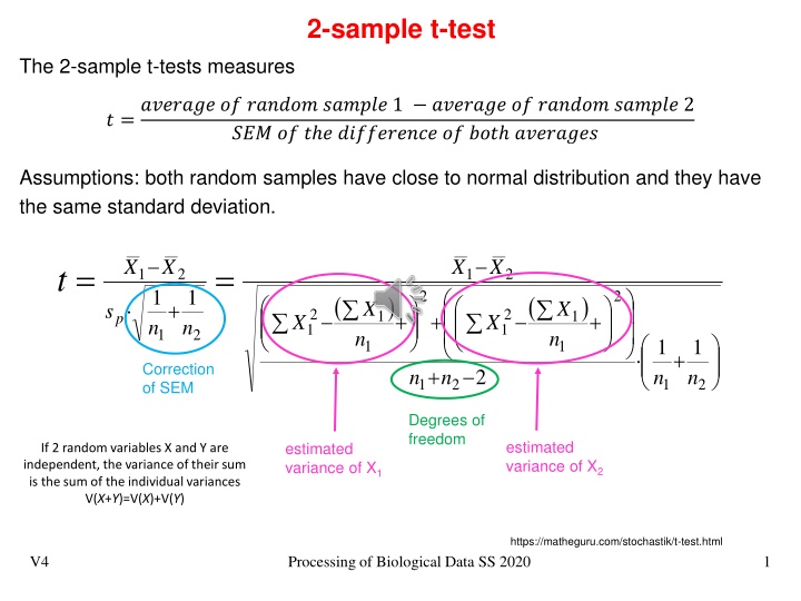
2-sample t-test The 2-sample t-tests measures ? =??????? ?? ?????? ?????? 1 ??????? ?? ?????? ?????? 2 ??? ?? ? ? ?????????? ?? ??? ???????? Assumptions: both random samples have close to normal distribution and they have the same standard deviation. 1 n X X X X = = t 1 2 1 2 1 n 2 2 ( ) ( ) + X X s 2 1 2 1 1 1 n + + + p X X n 1 2 n n 1 n 1 n 1 1 + Correction of SEM + 2 1 2 1 2 Degrees of freedom estimated variance of X2 estimated variance of X1 If 2 random variables X and Y are independent, the variance of their sum is the sum of the individual variances V(X+Y)=V(X)+V(Y) https://matheguru.com/stochastik/t-test.html V4 Processing of Biological Data SS 2020 1

Limma Package: Volcano plot The 'volcano plot' is an easy-to-interpret graph that summarizes both fold-change and t-test criteria. It is a scatter-plot of the negative log10- transformed p-values from the gene-specific t test against the log2 fold change. Genes with statistically significant differential expression according to the gene- specific t test will lie above a horizontal threshold line. Genes with large fold-change values will lie outside a pair of vertical threshold lines. The significant genes identified by the S, B, and regularized t tests will tend to be located in the upper left or upper right parts of the plot. Rapaport et al. (2013) Genome Biol. 14: R95 Cui & Churchill, Genome Biol. 2003; 4(4): 210 V4 Processing of Biological Data SS 2020 2

Detection of Outlier Samples/Genes V4 Processing of Biological Data SS 2020 3

Grubbs test Grubbs test can be used to test the presence of one outlier and can be used with data that is normally distributed (except for the outlier) and has at least 7 elements (preferably more). One tests the null hypothesis that the data has no outliers vs. the alternative hypothesis that there is one outlier. If you suspect that the maximum (minimum) value in the data set may be an outlier you can use the test statistic G x x x x = = max min or G SD SD The critical value for the test is ( ( ) 1 n t = crit + G ) crit 2 crit 2 n n t where tcritis the critical value of the t distribution T(n 2) and the significance level is /n. Thus the null hypothesis is rejected if G > Gcrit. http://www.real-statistics.com/students-t-distribution/identifying-outliers-using-t-distribution/grubbs-test/ V4 Processing of Biological Data SS 2020 4

GESD GESD was developed to detect 1 outliers in a dataset assuming that the body of its data points comes from a normal distribution. First, GESD calculates the deviation between every point xiand the mean , normalized by the standard deviation. At each iteration, it then removes the point with the maximum deviation. This process is repeated until all outliers that fulfill the condition identified where is the critical value calculated for all points using the percentage points of the t distribution. are V4 Processing of Biological Data SS 2020 5

GESD GESD and its predecessor ESD will always mark at least one data point as outlier even when there are in fact no outliers present. Therefore, using GESD to detect outliers in microarray data must be accompanied with a threshold of outlier allowance where a certain amount of outliers are detected before marking a gene as an outlier. The GESD method is said to perform best for datasets with more than 25 points. Additionally, the algorithm requires the suspected amount of outliers as an input. V4 Processing of Biological Data SS 2020 6

8.4 Detect outliers with MAD In contrast to GESD, the MAD algorithm (Rousseeuw and Croux 1993) is not based on the variance or standard deviation and thus makes no particular assumption on the statistical distribution of the data. At first, the raw median ?????? ? is computed over all data points. From this, MAD obtains the median absolute deviation (MAD) of single data points Xi from the raw median as: ??? = ? ?????? ?? ?????? ? b is a scaling constant. For normally distributed data, one uses b = 1.4826. As rejection criterion of outliers, one uses ?? ?????? ? ??? ? ??? ??? Suitable thresholds could be 3 (very conservative), 2.5 (moderately conservative) or 2 (poorly conservative). V4 Processing of Biological Data SS 2020 7

8.4 Detect outliers with MAD ??? = ? ?????? ?? ?????? ? Consider the data (1, 3, 4, 5, 6, 6, 7, 7, 8, 9, 100). It has a (raw) median value of 6. The absolute deviations ?? ?????? ? from 6 are (5, 3, 2, 1, 0, 0, 1, 1, 2, 3, 94). Sorting this list into (0, 0, 1, 1, 1, 2, 2, 3, 3, 5, 94) shows that the deviations have a median value of 2. When scaled with b = 1.4826, the median absolute deviation (MAD) for this data is roughly 3. Possible outliers above a rejection threshold would need to differ from the median by 6 to 9 or more. For this example, only the extreme data point (100) deviates that much. V4 Processing of Biological Data SS 2020 8

Simulated expression data sets Different gray levels represent different classes. Outlier cases are in black. SDS1/2 (left) has two known outliers (black) and 3 known switched samples. SDS3/4 (right) contain 50 outliers each. SDS1-3 follow Gaussian distributions while SDS4 follows a Poisson distribution. Barghash et al., J Proteomics Bioinform 2016, 9:2 V4 Processing of Biological Data SS 2020 9

Effect of 2 outliers on auto-correlation of a gene Effect of 2 introduced outlier points on co-expression analysis of a gene with itself (4 datasets from TCGA for COAD; GBM; HCC, OV tumor). X-axis : magnitude of perturbations applied as multiples of standard deviations (SD). For the smallest sample (COAD), two 2SD outliers, reduce the auto- correlation to 0.75. Barghash et al., J Proteomics Bioinform 2016, 9:2 V4 Processing of Biological Data SS 2020 10

Clustering dendogram Clustering dendrogram of dataset of simulated expression. Average Hierarchical Clustering bases on Euclidean distances (AHC-ED) clustered SDS1 into 3 main classes grouping the outlier samples (50 and 100) in a separate class. All switched samples marked by asterisks - were correctly clustered into their original classes. Barghash et al., J Proteomics Bioinform 2016, 9:2 V4 Processing of Biological Data SS 2020 11

Silhouette: validates clustering Large s(i) means good clustering Silhouette validation of the AHC-ED clustering of SDS1. The average distance of 0.36 indicates that AHC-ED succeeded in clustering SDS1. Silhouette coefficient: a(i) : average dissimilarity of i with all other data within the same cluster b(i) : lowest average dissimilarity of ito any other cluster, of which i is not a member Barghash et al., J Proteomics Bioinform 2016, 9:2 V4 Processing of Biological Data SS 2020 12

# of detected synthetic outlier data points (out of 50) Top: In normally distributed data, GESD identified largest number (46/50) of synthetic outliers. Bottom: If the two distributions have larger overlap (1 SD 2 SD 3 SD), detecting outliers becomes considerably harder. Barghash et al., J Proteomics Bioinform 2016, 9:2 V4 Processing of Biological Data SS 2020 13

MA quality control These authors compared four strategies of data analysis : - Strategy 1 No outlier removal - Strategy 2 Outlier removal guided by arrayQualityMetrics (outliers of boxplot) - Strategy 3 Removing random arrays (same number of arrays as in strategy 2) - Strategy 4 Array weights using the function arrayWeights from the limma Bioconductor package Kauffman, Huber (2010) Genomics 95, 138 V4 Processing of Biological Data SS 2020 14

Number of DE genes Data -> rma -> DE genes with moderated t-test in limma, FDR correction Number of differentially expressed genes identified: - on the whole dataset (white bars), - after removing outliers identified by arrayQualityMetrics (black bars) and - using weights obtained by arrayWeights from limma (grey bars). Many more DE genes identified after removing outlier genes. E-MEXP-170 has additional confounding effect of experiment date! This explains high # of DE genes. Kauffman, Huber (2010) Genomics 95, 138 V4 Processing of Biological Data SS 2020 15