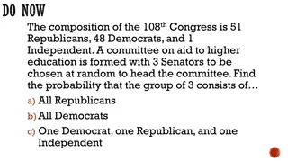
Explore the world of statistical distributions in this comprehensive guide. Learn about different types of distributions, their uses, and how to make accurate assumptions. Improve your ability to analyze data and make informed decisions.
Please find below an Image/Link to download the presentation.
The content on the website is provided AS IS for your information and personal use only. It may not be sold, licensed, or shared on other websites without obtaining consent from the author. If you encounter any issues during the download, it is possible that the publisher has removed the file from their server.
You are allowed to download the files provided on this website for personal or commercial use, subject to the condition that they are used lawfully. All files are the property of their respective owners.
The content on the website is provided AS IS for your information and personal use only. It may not be sold, licensed, or shared on other websites without obtaining consent from the author.
Objectives To develop the Black Belt s ability: to better identify different types of statistical distributions. to identify the uses of different distributions. to make assumptions given a known distribution. www.chools.in
Why Distributions? Base Line Calculations Normal Data: Z-Score gives Sigma Level. Non-Normal Data: Currently can only use discrete defect counts. Knowing the distribution can give us the same accuracy as for a normal distribution. Prediction What percent is above or below spec? Understanding What impact do distributions have on test statistics? www.chools.in
Distributions Exercise 1 Consider the following scenario: You need to estimate how well your Banking Center is doing in managing customer wait time. You gather a representative sample of 100 customer wait times. The data are in Distributions_Exercise_1.MTW. Given an upper specification limit of 5 minutes, calculate the sigma level of your process and the proportion of your customers that you predict will have to wait more than 5 minutes. www.chools.in
What is Probability? Probability of an outcome is a number that measures the likelihood that the outcome will occur when the experiment is performed. Example: In toss of a fair coin, probability of heads = 0.5 ( heads is 50% likely to occur). www.chools.in
What are Distributions? Probability distribution is a rule that specifies the possible outcomes and gives the probability of observing each of these values. Properties of a distribution: Probability of observing any particular value must be between 0 and 1. Sum of probabilities of all the values must equal 1. www.chools.in
What are Distributions? Properties of a distribution: The probability that any one of two or more values occurs is equal to the sum of their individual probabilities. P(X=1 or X=2) = P(X=1) + P(X=2) P( ) denotes probability of an outcome. X is known as a random variable. If X can take values 0, 1, 2, What is P(X 2)? How about P( 1 X 4)? www.chools.in
What are Distributions? Distributions for discrete random variables look different from distributions for continuous random variables. Normal Curve and Probability Areas 0.4 0.3 Discrete 0.2 0.1 0.0 Output Continuous www.chools.in
Discrete vs. Continuous Distributions Continuous Discrete Probability Density Function (PDF) The probability that a random variable has the value x, expressed in terms of an integral between two points. For example, the probability the x is between 3.15 and 3.25. Denoted by f(x) Probability Mass Function (PMF) The probability that a random variable takes the value x. For example, the probability that x is 3. Denoted by P(X=x) www.chools.in
Example: Discrete Probability Distribution This is the probability distribution for the number of heads expected when flipping a coin 10 times (binomial distribution): 0.25 0.20 probability 0.15 0.10 0.05 0 0 1 2 3 4 5 6 7 8 9 10 number of heads We can use this distribution to make predictions about coin flipping results: Probability of getting exactly 3 heads: P(x=3) = 0.117 = 11.7% Probability of getting 8 or more heads: P(x 8) = P(x=8) + P(x=9) + P(x=10) = 5.5% www.chools.in
Example: Continuous Probability Distribution The time it takes to process a credit card application may have a probability distribution that looks like this (Weibull distribution): Knowing the probability distribution allows us to make predictions, for example: The probability of taking between 8 and 12 days to process a credit card app is the area under the curve between 8 and 12. P(8 x 12) = 0.289 = 28.9% for the above distribution. www.chools.in
Cumulative Distribution Function Cumulative Distribution Function (CDF) the probability that a variable takes a value less than or equal to x. P(X x) for both discrete & continuous. F(x) is the area to the left of the vertical line at x F(x) www.chools.in
Common Probability Distributions Discrete Binomial Poisson Geometric Negative Binomial Hypergeometric Continuous Normal Exponential Weibull Chi Squared T F Lognormal Gamma Beta Not covered in this class. www.chools.in
Distribution Descriptions Parameters characterize the distributions. Location Parameter The lower or midpoint (as prescribed by the distribution) of the range of the random variable. E.g., for a normal distribution, the mean. Scale Parameter Determines the scale of measurement for x (magnitude of the x-axis scale). E.g., for a normal distribution, the standard deviation. Shape Parameter Defines the PDF shape within a family of shapes. E.g., for a t distribution, the degrees of freedom. www.chools.in
Normal Distribution GB training: focused on inferential statistics based on a normal distribution. N o rm a l C u r v e a n d P ro b a b ility A r e a s 0 .4 0 .3 68% 95% 0 .2 0 .1 99.73% 0 .0 - 2 -4 - 3 -1 0 2 4 1 3 Output www.chools.in
Normal Distribution (review) Population mean denoted by describes location Population standard deviation denoted by describes spread and scale Z score at a given value of interest x area from Z table x Z table shows the area under the curve from the Z score towards the right tail when Z is positive and toward the left tail when Z is negative. For Z = -2.5, explain what the value from Z table means (in terms of probability). www.chools.in
Z Table Exercise 1. Our teller drawers are supposed to have $1200 on average. If it goes to $1600, the teller should send some to the vault, or if it drops to $600, they should get currency from the vault. We take some measurements and find that the distribution is normal with an average of $945 and a standard deviation of $203. What is probability that a drawer is out of spec at any given time? 2. A sales manager randomly samples the average weekly sales of the sales force. The data form a normal distribution with an average of $6852 and a standard deviation of $986. What percent of the sales force is selling over $8,000 on any given week? In a group of 1,500 sales associates, how many associates will sell over $10,000? If we want to conduct special training for the bottom 20%, what is average sales of the associate at the 20thpercentile? www.chools.in
Applications of Normal Distribution Processes which have random variation about a target will typically be described mathematically by a normal distribution. This is the most commonly used probability distribution in Six Sigma. Uses of the normal distribution in Six Sigma include: Capability analyses. Hypothesis testing and confidence intervals. Central Limit Theorem. Control charts and out of control conditions. www.chools.in
Normal Distribution on Minitab To look up probabilities: Calc>Probability Distributions>Normal To fit distribution: Graph>Probability Plot To generate random data: Calc>Random Data>Normal www.chools.in
Exponential Distribution mean = st. dev. Another commonly used distribution is the exponential distribution. Some properties include: Maximum at x = 0, decays monotonically (steadily) as x increases. Approaches zero as x . Its mean is equal to its standard deviation. x must be non-negative. www.chools.in
Exponential Distribution Uses include probabilistic assessments of .. Mean time between failure (MTBF). Arrival times. Time, distance or space between occurrences of the events of interest. Queuing or wait-line Theories (Time between arrival of customers at a Banking Center). www.chools.in
Exponential Distribution on Minitab To look up probabilities: Calc>Probability Distributions>Exponential To fit distribution: Graph>Probability Plot>Exponential To generate random data: Calc>Random Data>Exponential www.chools.in
Weibull Distribution = 1 = 5 = 7 = 14 = 2 = 7 The Weibull is a family of distributions whose form varies greatly depending on its shape ( ) and scale ( ) parameters It is a catch-all distribution which should be used to describe data that has a single peak but is skewed (thus non-normal) Time studies very often result in a Weibull distribution. www.chools.in
Weibull Distribution on Minitab To look up probabilities: Calc>Probability Distributions>Weibull To fit distribution: Graph>Probability Plot>Weibull To generate random data: Calc>Random Data>Weibull www.chools.in
Example 1: Fitting Distributions with Minitab Minitab file DISTRIBUTIONS_EXAMPLE_1.MTW has three columns of data (A, B and C). Fit the appropriate distribution for A, B and C. Once you have found the appropriate distributions, for each of the distributions, determine: F(2.5) = P(X <= 2.5) Value of x when F(x) = 0.95 www.chools.in
Minitab Input Stat>Reliability/Survival>Distribution ID Plot-Right Cens . . . www.chools.in
Minitab Output Graphically, which looks like the best fit? Lowest Anderson- Darling statistic is the best fit. Which one is that? www.chools.in
Answering questions with data First determine location, shape and/or scale parameters. Graph>Probability Plot: Select Distribution www.chools.in
Answering questions with data Use these parameter values to determine probabilities: Calc>Probability Distributions>Weibull PDF: f(x) What is x for a given probability? CDF: F(x) Parameters Input x for PDF and CDF. Or input probability for the inverse cumulative probability. www.chools.in
Answering questions with data Cumulative Distribution Function Weibull with first shape parameter = 2.96574 and second = 4.48380 x P( X <= x ) 2.5000 0.1621 The probability that Process A will be below 2.5 is 16.21%. F(2.5) = 0.1621 Inverse Cumulative Distribution Function Weibull with first shape parameter = 2.96574 and second = 4.48380 P( X <= x ) x 0.9500 6.4911 For Process A, we have to get to 6.4911 to be assured we have captured 95% of the data. F(6.4911) = 0.95 Return to Slide 27 and repeat for Processes B and C. Return to Slide 4 and recalculate the sigma level. www.chools.in
Binomial Distribution Assumptions: Number of trials are fixed in advance. Just 2 outcomes for each trial. Trials are independent. Probability of an outcome does not change from trial to trial. www.chools.in
Binomial Distribution Uses include Estimating the probabilities of an outcome in any set of success or failure trials. Sampling for an attribute (acceptance sampling). Number of top two box ratings on a survey. Number of defective items in a batch size of n. www.chools.in
Binomial Distribution To look up Binomial Probabilities: Calc>Probability Distributions>Binomial Note: This is not PDF, it s probability P(X=x). CDF: F(x) What is x for a given probability? www.chools.in
Application of Binomial Distribution In a month-end report there is 1% probability of making an error in an expense figure. Every month 150 expense figures are presented in the report. You would like to know the probability that there will be any error in a report. An analyst would like to know the probability of 2 or more errors. www.chools.in
Application of Binomial Distribution (continued) n = 150 p = 0.01 Probability of no errors: P(0) = 22.1% Probability of one or more errors: P(x 1) = 1 P(0) = 77.9% Probability of exactly one error: P(1) = 33.6% Probability of two or more errors: P(x 2) = 1 [P(0) + P(1)] = 44.3% www.chools.in
Application of Binomial Distribution (continued) Minitab Output Probability Density Function Binomial with n = 150 and p = 0.0100000 x P( X = x ) 0.00 0.2215 Probability Density Function Binomial with n = 150 and p = 0.0100000 x P( X = x ) 1.00 0.3355 Cumulative Distribution Function Binomial with n = 150 and p = 0.0100000 x P( X <= x ) 1.00 0.5570 www.chools.in
Poisson Distribution Assumptions: Length of the observation period (or area) is fixed in advance. Events occurs at a constant average rate. Occurrences are independent. Number of occurrences in a time period. www.chools.in
Poisson Distribution Uses include Number of events in an interval of time (or area) when the events are occurring at a constant rate. Number of customer arrivals at a Banking Center. Design reliability tests where the failure rate is considered to be constant as a function of usage. www.chools.in
Poisson Distribution To look up Poisson Probabilities: Calc>Probability Distributions>Poisson Note: This is not PDF, it s probability P(X=x). CDF: F(x) What is x for a given probability? www.chools.in
Application of Poisson Distribution (continued) At a Banking Center, the customers arrive on average 2 per minute during the noon hour. The Banking Center manager needs your help in determining staffing level for this hour. She wants to know: What is the probability that there will be 4 or more arrivals between 12:00 and 12:01? www.chools.in
Application of Poisson Distribution (continued) Minitab Output Probability Density Function Probability Density Function Poisson with mu = 2.00000 Poisson with mu = 2.00000 x P( X = x ) x P( X = x ) 0.00 0.1353 3.00 0.1804 Probability Density Function Cumulative Distribution Function Poisson with mu = 2.00000 Poisson with mu = 2.00000 x P( X = x ) x P( X <= x ) 1.00 0.2707 3.00 0.8571 Probability Density Function Poisson with mu = 2.00000 x P( X = x ) 2.00 0.2707 www.chools.in