Statistical Mixing Model for Solution Behavior

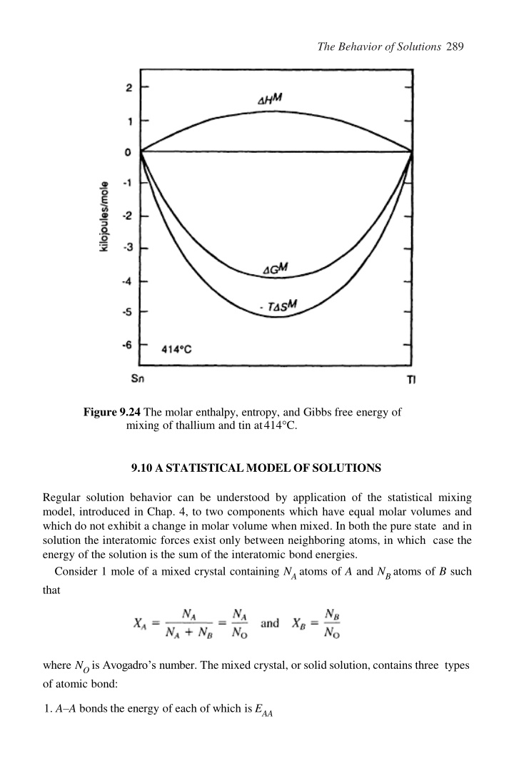
The Behavior of Solutions 289 Figure 9.24 The molar enthalpy, entropy, and Gibbs free energy of mixing of thallium and tin at414 C. 9.10 ASTATISTICALMODELOF SOLUTIONS Regular solution behavior can be understood by application of the statistical mixing model, introduced in Chap. 4, to two components which have equal molar volumes and which do not exhibit a change in molar volume when mixed. In both the pure state and in solution the interatomic forces exist only between neighboring atoms, in which case the energy of the solution is the sum of the interatomic bond energies. Consider 1 mole of a mixed crystal containing NAatoms of A and NBatoms of B such that where NO is Avogadro s number. The mixed crystal, or solid solution, contains three types of atomic bond: 1. A A bonds the energy of each of which is EAA

290 Introduction to the Thermodynamics ofMaterials 2. B B bonds the energy of each of which isEBB 3. A B bonds the energy of each of which isEAB By considering the relative zero of energy to be that when the atoms are infinitely far apart, the bond energies EAA, EBB, and EABare negative quantities. Let the coordination number of an atom in the crystal be z, i.e., each atom has z nearest neighbors. If, in the solution, there are PAAA A bonds, PB BB B bonds, and PABA B bonds, the energy of the solution, E, is obtained as the linear combination (9.78) and the problem of calculating E becomes one of calculating the values of PAA, PBB, and PAB. (The factor 2 arises because each A A bond involves two A atoms.)Thus or (9.79) Similarly, for B, NBz=PAB+2PBBor (9.80) Substitution of Eqs. (9.79) and (9.80) into Eq. (9.78)gives (9.81)

The Behavior of Solutions 291 Consider now the energies of the pure components before mixing. With NA atoms in pure A i.e., and similarly, for NB atoms in pure B Thus For the mixing process, from Eq.(5.10), and, as it has been stipulated that OVM=0,then (9.82) Eq. (9.82) shows that, for given values of E , E , and E , OHMdepends on P and AA BB AB AB further that, for the solution to be ideal, i.e., for OHM=0, (9.83)

292 Introduction to the Thermodynamics ofMaterials Thus, contrary to the preliminary discussion in Sec. 9.2 which suggested that ideal mixing required the condition EAB=EAA=EBB, it is seen that a sufficient condition is that E AB be the average of EAA and EBB. If |EAB|>|1/2(EAA+EBB|), then, from Eq. (9.82), OH is a negative quantity, corresponding to negative deviations from Raoultian ideal behavior, and, if |E |<|1/2(E +E )|, then OHM is a positive quantity, corresponding to AB AA BB positive deviations from Raoultian ideality. If OHM=0, then the mixing of the N with the N at oms of B is random, in which case A Eq. (9.45) gives M B In solutions which exhibit relatively small deviations from ideal behavior, that is |OHM| RT, it can be assumed that the mixing of the atoms is also approximately random, in which case PABcan be calculated as follows. Consider two neighboring lattice sites in the crystal labeled 1 and 2. The probability that site 1 is occupied by an A atomis and similarly, the probability that site 2 is occupied by a B atom is XB. The probability that site 1 is occupied by an A atom and site 2 is simultaneously occupied by a B atom is thus XAXB. But the probability that site 1 is occupied by a B atom and site 2 is simultaneously occupied by an A atom is also XAXB. Thus the probability that a neighboring pair of sites contains an A B pair is 2XAYB. By a similar argument, the probability that the neighboring sites contain an A A pair is and that the neighboring sites contain a B B pair is pair or an A A pair or a B B pairis . The probability that the neighboring sites contain an A B As the mole of crystal contain 1/2 zNO pairs of lattice sites,than

The Behavior of Solutions 293 i.e., (9.84) Similarly and Substituting Eq. (9.84) into Eq. (9.82)gives andif then (9.85) which shows that OHM is a parabolic function of composition. As random mixing is assumed, the statistical model corresponds to the regular solution model, i.e., (9.86)

294 Introduction to the Thermodynamics ofMaterials and thus (9.87) Application of Eq. (9.33a) to the heat of mixing gives and from Eq.(9.86) Thus (9.88a) and (9.88b) As the mixing is random,then andhence (9.89) But (9.90)

The Behavior of Solutions 295 comparison of which with Eq. (9.89) indicates that (9.91) The value of thus depends on the value of fi, which, in turn, is determined by the values of the bond energies EAA, EBB, and EAB. If fi is negative, then A<1, and if fi is positive, then A>1. Henry s law requires that A, and hence ln A, approach a constant value as XB approaches unity. Thus, as XB 1, ln being approached asymptotically. Similarly, in view of the relationship between Henry s and Raoult s laws, Raoult s law is approached asymptotically by the component i as Xi 1. The applicability of the statistical model to real solutions decreases as the magnitude of fi increases, i.e., if the magnitude of EABis significantly greater or less than the average of EAA and EBBthen random mixing of the A and B atoms cannot be assumed. The equilibrium configuration of a solution at constant T and P is that which minimizes the Gibbs free energy G, where G=H TS is measured relative to the unmixed components. As has been seen, minimization of G occurs as a compromise between minimization of H and maximization of S. If |EAB|>|1/2(EAA+EBB)| then minimization of H corresponds to maximization of the number of A B pairs (complete orderingof the solution). On the other hand, maximization of S corresponds to completely random mixing. Minimization of G thus occurs as a compromise between maximization of PAB(the tendency toward which increases with increasingly negative values of fi) and random mixing (the tendency toward which increases with increasing temperature). The critical parameters are thus fi and T, and, if fi is apprecia- bly negative and the temperature is not too high, then the value of PABwill be greater than that for random mixing, in which case the assumption ofrandom mixing isnot valid. Similarly, if |EAB|<|1/2(EAA+EBB)|, then minimization of H corresponds to min- imization of the number of A B pairs (complete clustering in the solution), and minimization of G occurs as a compromise between minimization of PAB(the tendency toward which increases with increasingly positive values of fi) and random mixing. Thus if fi is appreciably positive and the temperature is not too high, then the value ofPABwill be less than that for random mixing, in which case the assumption of random mixing is again invalid. In order for the statistical model, and hence the regular solution model, to be applicable, it is necessary that the above-mentioned compromise be such that the equilibrium solution configuration be not too distant from random mixing. As the entropy contribution to the Gibbs free energy is dependent on temperature, then , with this limitingvalue 1. For any value of fi, more nearly random mixing occurs as the temperature is increased, and

296 Introduction to the Thermodynamics ofMaterials 2. For any given temperature, more nearly random mixing occurs with smaller values of fi. The preceding discussion can be illustrated qualitatively by Fig. 9.25a and Fig. 9.25b. In these figures the x-axis represents the range of spatial configurations available to the atoms of a 50 mole percent A 50 mole percent B solution, quantified as the probability of the occurrence of an A B pair. The extreme configurations are complete clustering (A and B immiscible) in which the probability of the occurrence of an A B pair is zero, and the completely ordered structure in which the probability of the occurrence of an A B pair is unity. Random mixing occurs when the probability of the occurrence of an A B pair is 0.5. Movement along the x-axis from 0 to 1 occurs as follows. A and B atoms are exchanged to form dilute solutions of A in B and B in A and this process is continued until a single homogeneous solution is formed in which the probability of the occurrence of Figure 9.25 Illustration of the origins of deviation from regular solution behavior. an A B pair is less than 0.5. Thereafter the atoms are rearranged in such a manner as to continuously increase the probability of the occurrence of an A B pair to its limiting value of 1 in the completely ordered state. The change in the entropy of the system is given by the curve OSMin Fig. 9.25a and Fig. 9.25b; it increases from zero in the immiscible configuration, passes through a maximum at the random mixing decreases to zero in the ordered configuration. The corresponding variations of TOSMare shown in both figures. Fig. 9.25a is drawn for an exothermic solution and Fig. 9.25b is drawn for an endothermic solution. Thus, in Fig. 25a, the heat of mixing line, identified as OHM, begins at an arbitrary value of zero configuration and

The Behavior of Solutions 297 on the y-axis and decreases linearly with increasing probability of an A B pair. In Fig. 25b the OHM, begins at zero and increases linearly with increasing probability of an A B pair. The variations of the Gibbs free energy with configuration, given as the sum of OHM and TOSM, are shown as the lines OGM. The equilibrium configuration occurs at the position of the minimum on the OGMcurve, which is seen to be at a value of the probability of the occurrence of an A B pair of greater than 0.5 in the exothermically forming solution and at a value of less than 0.5 in the endothermically forming solution. It is seen that the random configuration is the equilibrium configuration only when OHM=0 and that, as the magnitude of |fi| for the system A B increases, then, at constant temperature, the position of the minimum in the OGMcurve moves further away from the random configuration. Similarly, for any given system (of fixed fi), as T, and hence |TOSM|, increases, the position of the minimum in the OGMcurve moves toward the random configuration. Figs. 9.25a and b also illustrate that both extreme configurations are physically unrealizable as, in order to have the minimum in the OGMcurve coincide with either extreme, infinite values of OHMwould be required (negative for complete ordering and positive for complete clustering). Similarly, with a non-zero OHMthe random configuration becomes the equilibrium configuration only at infinitetemperature. 9.11 SUBREGULAR SOLUTIONS In the regular solution model, the constant value of fi, which, via Eq. (9.85), gives a parabolic variation of OHM, and the ideal entropy of mixing lead to variations of GXSand OGMwhich are symmetrical about the composition X =0.5. The model can be made A more flexible by arbitrarily allowing fi to vary with composition suchas (9.92) and the so-called subregular solution model is that in which the values of all of the constants in Eq. (9.92), other than a and b, are zero. Thus, the subregular solution model gives the molar excess Gibbs free energy of formation of a binary A B solution as (9.93) Eq. (9.93) is an empirical equation, i.e., the constants a and b have no physical significance and are simply parameters the values of which can be adjusted in an attempt to fit the equation to experimentally measured data. The application of Eqs. (9.27a) and (9.27b) to Eq. (9.93) gives the partial molar excess Gibbs free energies of the components A and B as

298 Introduction to the Thermodynamics ofMaterials (9.94a) and (9.94b) The variations of GXS with X , with composition, for several combinations of a and b are B shown in Fig. 9.26. The maxima and/or minima in the curves occur at which, from Eq. (9.93), written as gives or

The Behavior of Solutions 299 Figure 9.26 Excess molar Gibbs free energy curves generated by the subregular solution model. Thus, as shown in Fig. 9.26a, with a=0, the minimum in the curve occurs at XB= 2/3, and with b=0 the solution behavior is regular. In Fig. 9.26e, with a=4000 J and b= 10,000 J, a maximum occurs in the curve at XB=0.17 and a minimum occurs at XB=0.76. The variation of fi with composition in the system Ag Au, obtained from the experimental measurements of Oriani at 1344 K, is shown in in Fig. 9.27.* Fitting these data to the subregular solution model with a= 13,465 J and b=5412.8 gives thevariation *R.A.Oriani, Thermodynamics of Liquid Ag Au and Au Cu Alloys and the Question of Strain Energy in Solid Solutions, Acta Met. (1956), vol. 4, p. 15.

300 Introduction to the Thermodynamics ofMaterials of OGM with composition shown by the line in Fig. 9.28. The open circles are experimentally measured values of OGM. The influence of temperature on the behavior of subregular solutions is accommodated by introducing a third constant, r, to give the molar excess Gibbs free energy of mixing as (9.95) The molar excess entropy of mixing is thus (9.96) and the molar heat of mixing (which is also the molar excess heat of mixing) is given by (9.97) 9.12 SUMMARY 1. Raoult s law is is said to exhibit Raoultian behavior. In all solutions, the behavior of the component i approaches Raoult s law as Xi 1. 2. Henry s law is pi=k Xi, and a component of a solution which conforms with this equation is said to exhibit Henrian behavior. In all solutions, the behavior of the component i approaches Henry s law as Xi 0. In a binary solution Henry s law is obeyed by the solute in that composition range over which Raoult s law is obeyed by the solvent. 3. The activity of the component i in a solution, with respect to a given standard state, is the ratio of the vapor pressure of i (strictly, the fugacity of i) exerted by the solution to the vapor pressure (the fugacity) of i in the given standard state. If the standard state is chosen as being pure i, then . An activity is thus , and a component of a solution that conforms with this law

The Behavior of Solutions 301 Figure 9.27 The variation, with composition, of fi, calculated from experimental measurements of OGM in the system Ag Au at 1350K. a ratio, and its introduction effects a normalization of the vapor pressure exerted by the component i in the solution. In terms of activity, Raoult s law is ai=Xi, and Henry s law is ai=kXi. 4. The difference between the value of an extensive thermodynamic property per mole of i in a solution, and the value of the property per mole of i in its standard state is called the partial molar property change of i for the solution process, i.e., if Q is any extensive thermodynamic property, the change in the property due to solution of 1 . In the case of Gibbs free energy mole of i is This difference in the molar Gibbs free energy is related to the activity of i in solution, . ln ai, and is called the partial with respect to the standard state, as molar Gibbs free energy of solution of i. The change in the Gibbs free energy accompanying the formation of 1 mole of solution from the pure components i (called the integral Gibbs free energy change) is , so that, for OGM=XA the binary A B, ln a , then OGM=RT(X ln a +X ln a ). In a A A A B B

302 Introduction to the Thermodynamics ofMaterials Raoultian solution, as a =X , then OGM=RT(X ln X +X ln X ). For any general i i A A B B extensive thermodynamic property 5. A Raoultian solution has the properties . (i.e., there is no change in (i.e., there is zero heat of volume when the components are mixed), mixing), and OGM,id=RT(X +X ln X ). As OSM,id= (6OGM,Bid/6T), OSM,id RZ X ln A B B = i i Xi, so that in a Raoultian solution, ln Xi. Figure 9.28 The subregular solution model fitted to experimental mea- surements of OGMin the system Ag Au at 1350 K as OGM=RT (XAgln XAg+XAuln XAu)+ (5,412.8XAu 13,465)XAuXAg. OSM,id is thus independent of temperature and is simply an expression for the maximum number of spatial configurations available to the system. 6. The thermodynamic behavior of non-Raoultian solutions is dealt with by introducing the activity coefficient, , which for the component i is defined as i= ai/Xi.The coefficient i, which, can have values of greater or less than unity, thus quantifies the deviation of i from Raoultian behavior. As ln ai= ln Xi+ln i, d ln . Thus if d /dT is positive,

The Behavior of Solutions 303 is negative and vice versa. The magnitude of the heat of formation of a nonideal solution is determined by the magnitudes of the deviations of the components of the solution from Raoultian behavior. Nonideal components approach Raoultian behavior with increasing temperature. Thus if i<1, then d i/dT is positive and if i,>1, d i/dT is negative. Solutions, the components of which exhibit negative deviations from Raoult s law, form exothermically, i.e., OHM<0, and vice versa. 7. The Gibbs-Duhem relationship is at constant temperature and pressure, where is the partial molar value of the extensive thermodynamic function Q of the solution component i. The excess value of an extensive thermodynamic property of a solution is the difference between the actual value and the value that the property would have if the components obeyed Raoult s law. Thus, for the general function Q, QXS=Q Qid, or for the Gibbs free energy, GXS=G Gid, or GXS=OGM OGM,id. As i ai/Xi, then G RT Z Xi ln i, 8. A regular solution is one which has an ideal entropy of formation and a non-zero heat of formation from its pure components. The activity coefficients of the components of a regular solution are given by the expression RT ln a (1 X )2, where a is a xs i i temperature-independent constant, the value of which is characteristic of particular solution. Thus ln ivaries inversely with temperature, and, as ln i, then is independent of temperature. Further-more, the heat of formation of a regular solution, being equal to GXS, is a parabolic function of composition, given by OHM=GXS=RTaX X =a X X . A B A B 9. Regular solution behavior is predicted by a statistical solution model in which it is assumed that the atoms mix randomly and that the energy of the solution is the sum of the individual interatomic bond energies in the solution. Random mixing can be assumed only if, in the system A B, the A B bond energy is not significantly different from the average of the A A and B B bond energies in the pure components. For any such deviation the validity of the assumption of random mixing increases with increasing temperature. The statistical model predicts tendency toward Raoultian behavior and Henrian behavior as, respectively, Xi 1 and as Xi 0. 10.The subregular solution model is one in which the value of T is assumed to be a linear function of composition, being given by fi=a+bXB. The variation of the molar excess Gibbs free energy of mixing is thus given by GXS=(a+ bX )X X . The B A B constants a and b are curve-fitting parameters and have no physical significance. 9.13 NUMERICALEXAMPLES Example 1 Copper and gold form complete ranges of solid solution at temperatures between 410 C

304 Introduction to the Thermodynamics ofMaterials and 889 C, and, at 600 C, the excess molar Gibbs free energy of formation of the solid solutions is given by Calculate the partial pressures of Au and Cu exerted by the solid solution of XCu= 0.6 at 600 C. From Eq. (9.87), the solid solutions are regular with fi= 28,280 J. Therefore, from Eq. (9.91), Thus, Similarly, Thus The saturated vapor pressure of solid copper is given by and the saturated vapor pressure of solid gold is given by Therefore, at 873K,

The Behavior of Solutions 305 and From Eq.(9.12), , and thus the partial pressures exerted by the alloyare and Example 2 At 700 K, the activity of Ga in a liquid Ga-Cd solution of composition XGa=0.5 has the value 0.79. On the assumption that liquid solutions of Ga and Cd exhibit regular solution behavior, estimate the energy of the Ga-Cd bond in the solution. The molar enthalpies of evaporation of liquid Ga and liquid Cd at their melting temperatures are, respectively, 270,000 and 100,000 J. With aGa=0.79 at XGa=0.5, Therefore, from Eq.(9.91), which gives At their melting temperatures, the coordination numbers of liquid Cd and liquid Ga are, respectively, 8 and 11. It will thus be assumed that the coordination number in the 50 50 solution is the average of 8 and 11, namely, 9.5. The bond energy, EGa Ga, is obtained from the molar enthalpy of evaporation, OHevap, according to

306 Introduction to the Thermodynamics ofMaterials The negative sign is required to conform with the convention that bond energies are negative quantities. Thus and similarly, The bond energy, ECd Ga, is obtainedfrom i.e., as PROBLEMS 1. One mole of solid Cr2O3at 2500 K is dissolved in a large volume of a liquid Raoultian solution of Al2O3 and Cr2O3 in which 2500 K. Calculate the changes in enthalpy and entropy caused by the addition. The normal melting temperature of Cr2O3 is 2538 K, and it can be assumed that the and which is also at . 2. When 1 mole of argon gas is bubbled through a large volume of an Fe-Mn melt of XMn=0.5 at 1863 K evaporation of Mn into the Ar causes the mass of the melt to decrease by 1.50 g. The gas leaves the melt at a pressure of 1 atm. Calculate the activity coefficient of Mn in the liquid alloy. 3. The variation, with composition, of GXS for liquid Fe Mn alloys at 1863 K is listed below. a. Does the system exhibit regular solution behavior?

The Behavior of Solutions 307 b. Calculate c. Calculate OGMat X and at XMn=0.6. =0.4. Mn d. Calculate the partial pressures of Mn and Fe exerted by the alloy of XMn=0.2. 4. Calculate the heat required to form a liquid solution at 1356 K starting with 1 mole of Cu and 1 mole of Ag at 298 K. At 1356 K the molar heat of mixing of liquid Cu and liquid Ag is given OHM= 20,590X X . Cu Ag 5. Melts in the system Pb-Sn exhibit regular solution behavior. At 473 C aPb= 0.055 in a liquid solution of XPb=0.1. Calculate the value of fi for the system and calculate the activity of Sn in the liquid solution of XSn=0.5 at 500 C. 6. The activities of Cu in liquid Fe-Cu alloys at 1550 C have been determined as Using, separately, Eqs. (9.55) and (9.61), calculate the variation of aFe with composition in the system at 1550 C. 9.7 The activities of Ni in liquid Fe-Ni alloys at 1600 C have been determined as Using, separately, Eqs. (9.55) and (9.61), calculate the variation of aFe with composition in the system at 1600 C. 9.8 Tin obeys Henry s law in dilute liquid solutions of Sn and Cd and the Henrian activity coefficient of Sn, , varies with temperature as Calculate the change in temperature when 1 mole of liquid Sn and 99 moles of liquid Cd are mixed in an adiabatic enclosure. The molar constant pressure heat capacity of the alloy formed is 29.5 J/K. 9.9 Use the Gibbs-Duhem equation to show that, if the activity coefficients of the components of a binary solution can be expressed as

308 Introduction to the Thermodynamics ofMaterials and over the entire range of composition, then a1= 1=0, and that, if the variation can be represented by the quadratic terms alone, then a2= 2. 9.10 The activity coefficient of Zn in liquid Zn Cd alloys at 435 C can be represented as Derive the corresponding expression for the dependence of In Cd on composition and calculate the activity of cadmium in the alloy of XCd=0.5 at 435 C. 9.11 The molar excess Gibbs free energy of formation of solid solutions in the system Au Ni be re presented by Calculate the activities of Au and Ni in the alloy of XAu=0.5 at 1100K.