Statistical Significance in Inference
Statistical significance plays a crucial role in inference, hypothesis testing, and estimation in the field of statistics. Learn about the historical aspect, basis of statistical inference, hypothesis testing, characteristics of hypotheses, null and alternative hypotheses, and more with informative images and explanations.

Download Presentation

Please find below an Image/Link to download the presentation.
The content on the website is provided AS IS for your information and personal use only. It may not be sold, licensed, or shared on other websites without obtaining consent from the author.If you encounter any issues during the download, it is possible that the publisher has removed the file from their server.
You are allowed to download the files provided on this website for personal or commercial use, subject to the condition that they are used lawfully. All files are the property of their respective owners.
The content on the website is provided AS IS for your information and personal use only. It may not be sold, licensed, or shared on other websites without obtaining consent from the author.
E N D
Presentation Transcript
Historical Aspect The term statistical significance was coined by Ronald Fisher(1890-1962). Student t-test : William Sealy Gosset. 2
Basis of Statistical Inference Statistical inference (a conclusion reached on the basis of evidence and reasoning)is the branch of statistics which is concerned with using probability concept to deal with uncertainly in decision making. It refers to the process of selecting and using a sample to draw inference about population from which sample is drawn. 3
Statistical Inference Testing of hypothesis Estimation of population value Point estimation Range estimation Mean, proportion estimation Confidence interval estimation 4
Hypothesis and its Testing Two Hypothesis are made to draw inference from Sample value- Null Hypothesis or hypothesis of no difference. Alternative Hypothesis of significant difference. A. B. The Null Hypothesis is symbolized as H0and Alternative Hypothesis is symbolized as H1orHA. In Hypothesis testing we proceed on the basis of Null Hypothesis. We always keep Alternative Hypothesis in mind. The Null Hypothesis and the Alternative Hypothesis are chosen before the sample is drawn. 5
Characteristics of Hypothesis Hypothesis should be clear and precise. 1. Hypothesis should be capable of being tested. 2. It should state relationship between variables. 3. It must be specific. 4. It should be stated as simple as possible. 5. It should be amenable to testing within a 6. reasonable time. It should be consistent with known facts. 7. 6
Null Hypothesis There is no difference between the operational procedures of open prostatectomy and TURP . There is no difference between open operation and transsphenoidal approach. There is no difference in the incidence of measles between vaccinated and non-vaccinated children. Drugs chloramphenicol is as good as drug cotrimoxazole in treating enteric fever. 7
Alternative Hypothesis Alternative Hypothesis of significant difference states that the sample result is different that is, greater or smaller than the hypothetical value of population. A test of significance such as Z-test, t-test, chi- square test, is performed to accept or reject the Null Hypothesis and accept theAlternative Hypothesis. 8
Interpreting the Result of Hypothesis The Hypothesis H0is true - our test accepts it because the result falls within the zone of acceptance at 5% level of significance. The Hypothesis H0is false our test rejects it because the estimate falls in the area of rejection. 9
Zones of acceptance and rejection Zone of acceptance - If the results of a sample falls in the plain area i.e. within the mean +/-1.96 standard error the Null Hypothesis is accepted- the area is called zone of acceptance. Zone of rejection - If the result of a sample falls outside the plain area, i.e. beyond mean +/-1.96 standard error, it is significantly different from population value. So Null Hypothesis is rejected and alternative hypothesis is accepted. This area is called zone of rejection. 10
Setting a criteria Accept H0 Null Hypothesis Reject H0 Reject H0 H0 Zcrit Zcrit 11
Type 1 and Type 2 Error When a Null Hypothesis is tested, there may be four possible outcomes: A. The Null Hypothesis is true but our test rejects it. B. The Null Hypothesis is false but our test accepts it. C. The Null Hypothesis is true and our test accepts it. D. The Null Hypothesis is false but our test rejects it. Type 1 Error rejecting Null Hypothesis when Null Hypothesis is true. It is called error . Type 2 Error accepting Null Hypothesis when Null Hypothesis is false. It is called -error . 12
Type 1 and Type 2 Error Decision Chart Decision Accept H0 Reject H0 H0true Correct decision Type 1 error H0false Type 2 error Correct decision 13
Type 1 and Type 2 Error The Null Hypothesis is True 1- (confidence level) False (type 2 error) Accept if p>=0.05(non- significant) conclusion- negative Reject if p<0.05(significant ) conclusion- positive (type 1 error) 1- (power of the test) 14
P-value The probability of committing Type 1 Error is called the P-value. Thus p-value is the chance that the presence of difference is concluded when actually there is none. When the p-value is between 0.05 and 0.01 the result is usually called significant. When p value is less than 0.01, result is often called highly significant. When p value is less than 0.001 and 0.005, result is taken as very highly significant. 15
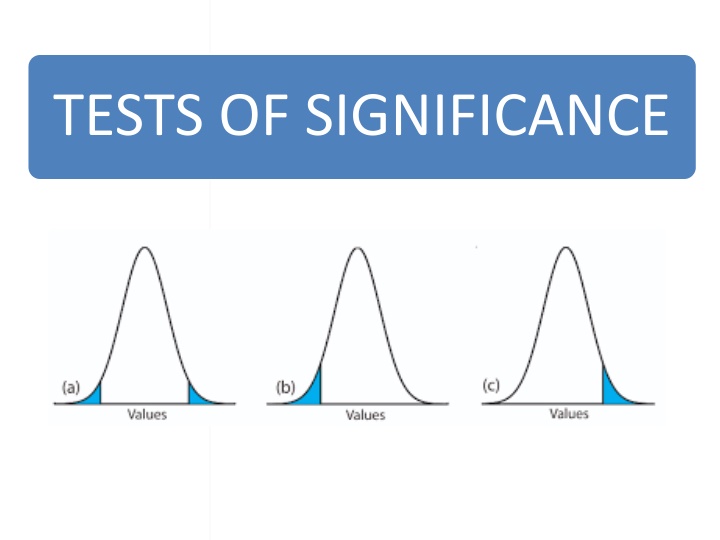
ONE-TAILED TEST If HA states is < some value, critical region occupies left tail. If HA states is > some value, critical region occupies right tail. 16
RIGHT-TAILED TEST H0: = 100 H1: > 100 Points Right Fail to rejectH0 Reject H0 alpha Values that differ significantly from 100 Zcrit 100 17
LEFT-TAILED TESTS H0: = 100 H1: < 100 Points Left Reject H0 Fail to reject H0 alpha Values that differ significantly from 100 100 Zcrit 18
TWO-TAILED HYPOTHESIS TESTING HA is that is either greater or less than H0 HA: H0 is divided equally between the two tails of the critical region. 19
TWO-TAILED HYPOTHESIS TESTING H0: = 100 H1: 100 Means less than or greater than Reject H0 Fail to reject H0 Reject H0 alpha 100 Zcrit Zcrit Values that differ significantly from 100 20
Parametric vs. Non-parametric Tests Not based on any particular parameter such as mean Do not require that the means follow a particular distribution such as Gaussian. Used when the underlying distribution is far from Gaussian (applicable to almost all levels of distribution) and when the sample size is small Based on specific distribution such as Gaussian 21
Parametric Tests 1. Student s t- test(one sample, two sample, and paired) 2. Z test ANOVA F-test 3. Pearson s correlation(r) Non-Parametric Tests 1. Sign test(for paired data), Wilcoxon Signed-Rank test for matched pair, Wilcoxon Rank Sum test (for unpaired data) 2. Chi-square test Spearman s Rank Correlation (p), ANOCOVA 3. Kruskal-Wallis test 22
Purpose of application Parametric test Non-Parametric test Comparison of two independent groups. t -test for independent samples Wilcoxon rank sum test Test the difference between paired observation Comparison of several groups t -test for paired observation Wilcoxon signed-rank test ANOVA Kruskal-Wallis test Quantify linear relationship between two variables Test the association between two qualitative variables Pearson s Correlation Spearman s Rank Correlation _ Chi-square test 23
Types of Parametric Tests 1. Students t-tests - A statistical criterion to test the hypothesis that mean is superficial value, or that specified difference, or no difference exists between two means. It requires Gaussian distribution of the values, but is used when SD is not known. 2. Proportion test (z-score) - A statistical test of hypothesis based on Gaussian distribution, generally used to compare two means or two proportions in large samples, particularly when the SD is known. 3. ANOVA F-test Used when the number of groups compared are three or more and when the objective is to compare the means of a quantitative variable. 24
Types of t-tests (student t test) One sample only one group is studied and an externally determined claim is examined. Two sample there are two groups to compare. Paired used when two sets of measurements are available, but they are paired . 25
Steps of t-tests (student t test) Find the difference between the actually observed mean and the claimed mean. Estimate the standard error (SE) of mean by S/n, where s is the standard deviation and n is the number of subjects in the actually studied sample. The SE measures the inter-sample variability Check the difference obtained in step 1 is sufficiently large relative to the SE. for this, calculate students t. this is called the test criterion. Rejection or non-rejection of the null depends on the value of this t . Reject the null hypothesis if the t-value so calculated is more than the critical value corresponding to the pre-fixed alpha level of significance and appropriate df. 26
Steps of paired t-test Obtain the difference for each pair and test the null hypothesis that the mean of these differences is zero (this null hypothesis is same as saying that the means before and after are equal). For paired samples : t = d/(Sd/(n)^1/2) d : is the sample mean of the differences Sd : is standard deviation.
z test The z-test is a hypothesis test to determine if a single observed mean is significantly different (or greater or less than) the mean under the null hypothesis, when you know the standard deviation of the population. 30
The observed value of z is 2013 which is greater than the critical value of 1.64. therefore, we reject H0.
Chi-square Test A statistical test that researchers use to determine if their experimental data supports (or doesn t support) the hypothesis being tested. Chi-square gives a measure of goodness of fit which defines how well data that was expected from their hypothesis fits with what was actually observed in their experiment. The chi-square (X2) method allows researchers to assess what is called the "goodness of fit" between expected and observed values.
Chi-square (2) Test There are two types of chi-square analysis methods: 1. goodness of fit (hypothesis testing) 2. Chi-square test for independence (which determines if there is an association between variables).
Example chi-square test Tomato bacterial spot disease To figure out what phenotypic classes are expected and the number of individual plants in each class. Based upon the observations in the F1where all showed resistance, test the hypothesis that resistance is controlled by one dominant gene. Therefore, for the 197 plants in F2generation of selfing the F1s from the 6.8068 x OH88119 cross, expected 147.75 tomato plants to be resistant to bacterial spot and 49.25 to be susceptible.
Chi-square Test The formula for calculating the X2value is: X2 = (observed expected)2/ expected
Interpreting the results of our chi-square calculation. For this, we will need to consult a Chi-Square Distribution Table. This is a probability table of selected values of X2(next slide). Statisticians calculate certain possibilities of occurrence (P values) for a X2value depending on degrees of freedom. Degrees of freedom is simply the number of classes that can vary independently minus one, (n-1). In this case the degrees of freedom = 1, because we have 2 phenotype classes: resistant and susceptible. If chi-square calculated value is greater than the chi-square critical value, then you reject your null hypothesis. If your chi-square calculated value is less than the chi-square critical value, then you "fail to reject your null hypothesis.
Finding the probability value for a chi-square of 1.2335 with 1 degree of freedom. First read down column 1 to find the 1 degree of freedom row and then go to the right to where 1.2335 would occur. This corresponds to a probability of less than 0.5 but greater than 0.25, as indicated by the blue arrows. we failed to reject our hypothesis that resistance to bacterial spot in this set of crosses is due to a single dominantly inherited gene.
Analysis of Variance Analysis of variance (ANOVA) is a statistical technique that is used to check if the means of two or more groups are significantly different from each other. ANOVA checks the impact of one or more factors by comparing the means of different samples. We can use ANOVA to prove/disprove if all the medication treatments were equally effective or not.
A t-test is also used to compare the samples. When we have only two samples, t-test and ANOVA give the same results. However, using a t-test would not be reliable in cases where there are more than 2 samples. If we conduct multiple t-tests for comparing more than two samples, it will have a compounded effect on the error rate of the result.
Analysis of Variance The analysis of variance (ANOVA) is a statistical tool that has two common applications in context to plant breeding. First, ANOVA can be used to test for differences among treatment means in an experiment. Common examples of treatments are genotype, location, and variety. Second, ANOVA can be used to aid in estimates of heritability by partitioning variances. This module focuses on simple ANOVA models to evaluate differences between treatments.
In ANOVA, the total variance of all samples is calculated. Portions of the total variance can be attributed to known causes (e.g., genotype). This leaves a residual portion of the variance that is uncontrolled or unexplained and is referred to as experimental error. In the simplest case, linear equations can be developed to describe the relationship between a trait and treatment. The question can then be asked, "which linear equation best fits the data for each treatment?" These linear equations take the following form: Y = (m) + f(treatment) + error where Y is equal to the trait value (m) is the population mean f(treatment) is a function of the treatment error represents the residual
F-Statistic The statistic which measures if the means of different samples are significantly different or not is called the F- Ratio. Lower the F-Ratio, more similar are the sample means. In that case, we cannot reject the null hypothesis. F = Between group variability / Within group variability If between group variability increases, sample means grow further apart from each other. In other words, the samples are more probable to be belonging to totally different populations.
The F-statistic calculated can be compared with the F-critical value for making a conclusion. If the value of the calculated F-statistic is more than the F-critical value (for a specific /significance level), then we reject the null hypothesis and can say that the treatment had a significant effect.
Example: One-way ANOVA Excel File
Two-way ANOVA A Two Way ANOVA is an extension of the One Way ANOVA. With a One Way, you have one independent variable affecting a dependent variable. With a Two Way ANOVA, there are two independents. Use a two way ANOVA when you have one measurement variable (i.e. a quantitative variable) and two nominal variables. In other words, if your experiment has a quantitative outcome and you have two categorical explanatory variables, a two way ANOVA is appropriate
Multivariate Analysis (MANOVA) Analysis of variance (ANOVA) tests for differences between means. MANOVA is just an ANOVA with several dependent variables. It s similar to many other tests and experiments in that it s purpose is to find out if the response variable (i.e. your dependent variable) is changed by manipulating the independent variable. The test helps to answer many research questions, including: Do changes to the independent variables have statistically significant effects on dependent variables? What are the interactions among dependent variables? What are the interactions among independent variables?


")


 Test")


")