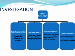
Statistics Essentials for Performance Analysis

Summarizing Measured Data Andy Wang CIS 5105 Computer Systems Performance Analysis

Introduction to Statistics Concentration on applied statistics Especially those useful in measurement Today s lecture will cover 15 basic concepts You should already be familiar with them

1. Independent Events Occurrence of one event doesn t affect probability of other Examples: Coin flips Inputs from separate users Unrelated traffic accidents What about second basketball free throw after the player misses the first?

2. Random Variable Variable that takes values probabilistically Variable usually denoted by capital letters, particular values by lowercase Examples: Number shown on dice Network delay

3. Cumulative Distribution Function (CDF) Maps a value a to probability that the outcome is less than or equal to a: ( ) ( x a x P a F = ) Valid for discrete and continuous variables Monotonically increasing Easy to specify, calculate, measure

CDF Examples Coin flip (T = 0, H = 1): 1 0.5 0 0 1 2 3 Exponential packet interarrival times: 1 0.5 0 0 1 2 3 4

4. Probability Density Function (pdf) Derivative of (continuous) CDF: x dF x f ) ( = ( ) dx Usable to find probability of a range: = P ( x x x ) F ( x ) F ( x ) 1 2 2 1 x = 2 f ( x ) dx x 1

Examples of pdf Exponential interarrival times: 1 0 0 1 2 3 Gaussian (normal) distribution: 0.45 0.4 0.35 0.3 0.25 0.2 0.15 0.1 0.05 0 -3 -2 -1 0 x 1 2 3

5. Probability Mass Function (pmf) CDF not differentiable for discrete random variables pmf serves as replacement: f(xi) = pi where piis the probability that x will take on the value xi = ( ) ( 2 1 F x x x P ) ( ) x F x 2 1 x = p i x x 1 2 i

Examples of pmf 1 Coin flip: 0.5 0 0 1 Typical CS grad class size: 0.5 0.4 0.3 0.2 0.1 0 4 5 6 7 8 9 10 11

6. Expected Value (Mean) n = i Mean (mu) = = = E ( x ) p x xf ( x dx ) i i 1 Summation if discrete Integration if continuous

7. Variance n = i Var(x) = = 2 2 E [( x ) ] p ( x ) i i 1 + = 2 ( x ) f ( x dx ) i Often easier to calculate equivalent 2 2 ) ( ) ( x E x E Usually denoted 2; square root (sigma) is called standard deviation

8. Coefficient of Variation (C.O.V. or C.V.) Ratio of standard deviation to mean: = C.V. Indicates how well mean represents the variable Does not work well when 0

9. Covariance Given x, y with means xand y, their covariance is: ) , ( Cov y x xy = = = 2 E [( x )( y )] x y E ( xy ) E ( x ) E ( y ) High covariance implies y departs from mean whenever x does

Covariance (contd) For independent variables, E(xy) = E(x)E(y) so Cov(x,y) = 0 Reverse isn t true: Cov(x,y) = 0 doesn t imply independence If y = x, covariance reduces to variance

10. Correlation Coefficient Normalized covariance (rho): 2 ??? ???? ??????????? ?,? = ???= Always lies between -1 and 1 Correlation of 1 x ~ y, -1 ~ x y

11. Mean and Variance of Sums For any random variables, ( 2 2 1 1 E a x E a + = + + + E a x a x a x ) + k + k ( ) ( x ) a E ( x ) 1 1 2 2 k k For independent variables, ( Var 1 1 x a = + + + a x a x a x ) 2 + 2 a k k 2 1 2 2 + + 2 k Var ( ) V ar ( x ) a V ar ( x ) 1 2 k

12. Quantile x value at which CDF takes a value is called -quantile or 100 -percentile, denoted by x . = ) ( ) ( x F x x P = If 90th-percentile score on GRE was 162, then 90% of population got 162 or less

Quantile Example 1.5 1 0.5 0 0 2 0.5-quantile -quantile

13. Median 50th percentile (0.5-quantile) of a random variable Alternative to mean By definition, 50% of population is sub- median, 50% super-median Lots of bad (good) drivers Lots of smart (not so smart) people

14. Mode Most likely value, i.e., xi with highest probability pi, or x at which pdf/pmf is maximum Not necessarily defined (e.g., tie) Some distributions are bi-modal (e.g., human height has one mode for males and one for females) Can be applied to histogram buckets

Examples of Mode Mode 0.2 Dice throws: 0.1 0 2 3 4 5 6 7 8 9 10 11 12 Mode Adult human weight: Sub-mode

15. Normal (Gaussian) Distribution Most common distribution in data analysis pdf is: 1 ) ( 2 ( x ) = 2 f x e 2 2 - x + Mean is , standard deviation

Notation for Gaussian Distributions Often denoted N( , ) Unit normal is N(0,1) If x has N( , ), has N(0,1) x The -quantile of unit normal z ~ N(0,1) is denoted z so that x z = + = P ( ) z P ( x )

Why Is Gaussian So Popular? We ve seen that if xi ~ N( , ) and all xi independent, then ixi is normal with mean i i and variance = i2 i2 Sum of large no. of independent observations from any distribution is itself normal (Central Limit Theorem) Experimental errors can be modeled as normal distribution.

Summarizing Data With a Single Number Most condensed form of presentation of set of data Usually called the average Average isn t necessarily the mean Must be representative of a major part of the data set

Indices of Central Tendency Mean Median Mode All specify center of location of distribution of observations in sample

Sample Mean Take sum of all observations Divide by number of observations More affected by outliers than median or mode Mean is a linear property Mean of sum is sum of means Not true for median and mode

Sample Median Sort observations Take observation in middle of series If even number, split the difference More resistant to outliers But not all points given equal weight

Sample Mode Plot histogram of observations Using existing categories Or dividing ranges into buckets Or using kernel density estimation Choose midpoint of bucket where histogram peaks For categorical variables, the most frequently occurring Effectively ignores much of the sample

Characteristics of Mean, Median, and Mode Mean and median always exist and are unique Mode may or may not exist If there is a mode, may be more than one Mean, median and mode may be identical Or may all be different Or some may be the same

Mean, Median, and Mode Identical Median Mean Mode pdf f(x) x

Median, Mean, and Mode All Different pdf f(x) Mode Mean Median x

So, Which Should I Use? If data is categorical, use mode If a total of all observations makes sense, use mean If not, and distribution is skewed, use median Otherwise, use mean But think about what you re choosing

Some Examples Most-used resource in system Mode Interarrival times Mean Load Median

Dont Always Use the Mean Means are often overused and misused Means of significantly different values Means of highly skewed distributions Multiplying means to get mean of a product Example: PetsMart Average number of legs per animal Average number of toes per leg Only works for independent variables Errors in taking ratios of means Means of categorical variables

Example: Bandwidth Experiment number File size (MB) Transfer time (sec) Bandwidth (MB/sec) 1 2 20 20 1 2 20 10 What is the average bandwidth? (20 MB/sec + 10 MB/sec)/2 = 15 MB/sec ???

Example: Bandwidth Experiment number File size (MB) Transfer time (sec) Bandwidth (MB/sec) 1 2 20 20 1 2 20 10 When file size is fixed Average transfer time = 1.5 sec Average bandwidth = 20 MB / 1.5 sec = 13.3 MB/sec (11% difference!) Another way (20MB + 20MB)/(1 sec + 2 sec) = 13.3 MB/sec

Example 2: Same Bandwidth Numbers Experiment number File size (MB) Transfer time (sec) Bandwidth (MB/sec) 1 2 60 20 3 2 20 10 (60MB + 20MB)/(3 sec + 2 sec) = 16 MB/sec

Example 2: Bandwidth Experiment number File size (MB) Transfer time (sec) Bandwidth (MB/sec) 1 2 20 60 1 6 20 10 (60MB + 20MB)/(1 sec + 6 sec) = 11 MB/sec

Geometric Means An alternative to the arithmetic mean ( i 1 = ) / 1 n n = x ix Use geometric mean if product of observations makes sense

Good Places To Use Geometric Mean Layered architectures Performance improvements over successive versions Average error rate on multihop network path

Harmonic Mean Harmonic mean of sample {x1, x2, ..., xn} is n x 1 1 2 1 = 1 + + + x x n x Use when arithmetic mean of 1/x1 is sensible

Example of Using Harmonic Mean When working with MIPS numbers from a single benchmark Since MIPS calculated by dividing constant number of instructions by elapsed time m ti xi = Not valid if different m s (e.g., different benchmarks for each observation)

Another Example of Using Harmonic Mean Bandwidth from a given benchmark Constant number of bytes (B) divided by varying elapsed times (t1, t2 ) B/t1, B/t2, We really want to average the times first T = (t1 + t2 .)/n Then compute the bandwidth B/T = Bn/(t1 + t2 ) = n/(t1/B + t2/B .)

Means of Ratios Given n ratios, how do you summarize them? Can t always just use harmonic mean Or similar simple method Consider numerators and denominators

Considering Mean of Ratios: Case 1 Both numerator and denominator have physical meaning Then the average of the ratios is the ratio of the averages

Example: CPU Utilizations Measurement Duration 1 1 1 1 100 Sum Mean? Busy (%) 40 50 40 50 20 200 % CPU

Mean for CPU Utilizations Measurement Duration 1 1 1 1 100 Sum Mean? Busy (%) 40 50 40 50 20 200 % Not 40% CPU

Properly Calculating Mean For CPU Utilization Why not 40%? Because CPU-busy percentages are ratios So their denominators aren t comparable The duration-100 observation must be weighted more heavily than the duration-1 observations