Study Notes: Probe Inductance in Coax-Fed Patch Waveguide
Explore detailed study notes on probe inductance in a coax-fed patch waveguide. Learn about the probe model, calculations, and theoretical solutions for understanding parallel-plate waveguide systems.

Download Presentation

Please find below an Image/Link to download the presentation.
The content on the website is provided AS IS for your information and personal use only. It may not be sold, licensed, or shared on other websites without obtaining consent from the author. If you encounter any issues during the download, it is possible that the publisher has removed the file from their server.
You are allowed to download the files provided on this website for personal or commercial use, subject to the condition that they are used lawfully. All files are the property of their respective owners.
The content on the website is provided AS IS for your information and personal use only. It may not be sold, licensed, or shared on other websites without obtaining consent from the author.
E N D
Presentation Transcript
ECE 6345 Spring 2024 Prof. David R. Jackson ECE Dept. Notes 5 1
Overview This set of notes discusses the probe inductance of a coax-fed patch. Introduce probe model for a parallel-plate waveguide Use this model to calculate the probe inductance 2
Probe Inductance Probe Patch Parallel-Plate Waveguide Model z 2a , h r r x 3
Probe Inductance The probe current is assumed to be uniform in the z direction, and the metal is removed by the equivalence principle. Radiation from the coax frill is neglected. = 0 Assume that z z = k k 0 r r 2a , h 0I r r = r x 0 r a Hollow tube of uniform surface current I = 0 J sz 2 a 4
Probe Inductance (cont.) = = ( ) = z E E 0 0 Assume since z z 2 2 + = 0 E k E z z General solution: ( ) J k cos( sin( ) k z k z cos( sin( ) n n n z = E z ) ( ) ) Y k n z ( m ) 1/2 2 2 z Choose = = = 0, 0 m n k k k = k z h 5
Probe Inductance (cont.) Hence ( ( ) ) J k Y k finite at the origin infinite at the origin 0 = E z 0 or ( ) 1 0 2 0 ( ) H k incoming wave = E z ( ) ( ) H k outgoing wave ( ) ( ) z ( ) ( ) z ( ) 1 n + ( ) z H J z jY z n n ( ) 2 n ( ) z H J jY n n 6
Probe Inductance (cont.) y Model: I 0 = [A/ m] J sz J 2 a sz a x , r r Hollow tube of current Note: The tube may be thought of as being infinite in the z direction (image theory). 7
Probe Inductance (cont.) y = A J k a Model: 0( ) E z J sz a x + + (2) 0( = k a ) E A H z , r r + = = E E a (BC #1) z z I 0 = [A/ m] J + = H H J (BC #2) sz 2 a sz 8
Probe Inductance (cont.) + (2) 0 = BC 1: ( ) ( ) A J ka A H ka = A J k a 0( ) E 0 z 1 ( ) = BC 2: H E j + + E (2) 0( = k 1 E a ) E A H z = z j z 1 E z = j + = = E E a (BC 1) so z z + = H H J (BC 2) I k sz + (2) 0 0 = ( ) ( ) A H ka A J ka 0 2 j a 9
Probe Inductance (cont.) Hence, eliminating A- using BC 1, we have: (2) 0 J ka ( ) H ka I j + + (2) 0 0 = ( ) ( ) A H ka A J ka 0 ( ) 2 a k 0 or I j + (2) 0 (2) 0 0 = ( ) ( ) ( ) ( ) ( ) A J ka H ka J ka H ka J ka 0 0 0 2 a k 10
Probe Inductance (cont.) Wronskian Identity: 2 ( ) x (2) n (2) n = ( ) x H ( ) x H ( ) x J J j n n x Hence + I 2 ka j 0 = ( ) A j J ka ( ) 0 2 a k or I ( ) + 0 = 0( ) A J ka 4 I = + k 0 = 0( ) so A k J ka Next, use 4 11
Probe Inductance (cont.) Hence I + (2) 0 0 = ( ) ( ) E k J ka H k 0 z 4 z 2a , h r r I Next, we use x h E V I z = a = = Z in I 0 0 ( ) kh (2) 0 so = ( ) ( ) Z J ka H ka in 0 4 Note: The imaginary part of Zin should be fairly accurate for the probe feed of a patch, but not the real part (the radiation effects are very different). 12
Probe Inductance (cont.) We could also complex power: 2 cP z = Z in 2 ( ) 0 I 2a , h r r I 1 x * s i = E J dS P c 2 s 2 h 1 ( ) = kh * i zs ( ) E a J adzd (2) 0 z = 2 ( ) ( ) Z J ka H ka 0 0 in 0 4 h = * i zs ( ) a E a J dz z 0 a (same result) h = * 0 ( ) E a I dz z 2 1 2 1 8 a 0 I ( ) I h = (2) 0 * 0 ( ) ( ) 0 k J ka H ka dz 0 4 0 ( ) = k J ka H 2 0 (2) 0 ( ) ( ) I h ka 0 13
Probe Inductance (cont.) ( ) kh ( ) = ( ) X J ka Y ka Taking the imaginary part: in 0 0 4 ( ) (2) 0( = ) ( ) ( ) H ka J ka jY ka Recall: 0 0 ka 1 For 2 ka + J ka ( ) ln Y ka 0( ) 1 0 2 0.57722 ( ) where Euler's constant 14
Probe Inductance (cont.) Approximating the Y0Bessel function, we have: 2 ka kh = + ln X in 2 or 2 ( ) = + ln 0 X k h r in 0 r r 2 k a r 0 r r or 2 ( ) = + 0 ln X k h in 0 r 2 k a 0 r r 15
Probe Inductance (cont.) We then have (with Xin = Xp): 2 ( ) = + ln 0 X k h ( ) 0 p r 2 k a 0 r r Alternative form: 2 h = + ln X ( ) 0 p r k a 0 0 r r 376.7303 0.57722 ( ) Euler's constant 0 16
Probe Inductance (cont.) X X k X k c p p p We can solve for the probe inductance using = = = L 0 0 p 0 0 2 H = + ln 0 L h ( ) p r 2 c k a 0 r r 2 ( ) = ln ln 0 0 L h h k a 0 p r r 2 2 c c r r The probe inductance is slightly dependent on frequency. = = 2 f In practice, we can evaluate it using 0 0 17
Probe Inductance (cont.) Example = 2.94 0.1524 [cm] r ( ( ( ) = = = 60mils = h ) 0.0635 [cm] 50[ ] a SMAConnector ) 2.0 [GHz] 14.9896 [cm] f 0 X = 12.3 [ ] p H 10 = = 9.79 10 0.979 [nH] L p 18
Probe Inductance (cont.) Results: Probe Reactance (Xf= Xp= Lp) 40 = 2.2 = r 35 / 1.5 W L h a CAD exact Rectangular patch = 0.0254 0.5mm = 30 0 25 Xf ( ) y 20 CAD: 15 2 (x0, y0) ( ) = + ln 0 X k h W ( ) 0 p r 2 k a 10 0 r r ( ) 2 / 1 rx x L 0 5 L x Exact: L 0 The cavity model for Xp with all infinite modes (excluding the (1,0) term). 0 0.1 0.2 0.3 0.4 0.5 Xr 0.6 0.7 0.8 0.9 1 rx Center Edge The normalized feed location ratio xr is zero at the center of the patch (x = L/2), and is 1.0 at the patch edge (x = L). 19 19
Image Correction to Probe Inductance Image Theory Image theory can be used to improve the simple parallel-plate waveguide model when the probe gets close to the patch edge. PMC Wall Image Currents The probe images are reflections of the original probe current about the four PMC walls. s 2a S = distance from probe to left PMC wall. P Pr ri im ma ar ry y c cu ur rr re en nt t Using image theory, we have an infinite set of image probes. We will just worry about the image that is closest to the original probe current. 20
Image Correction to Probe Inductance (cont.) A simple approximate formula is obtained by using two terms: the original probe current in a parallel- plate waveguide and one image. This should be an improvement when the probe is close to an edge. + two p image p X = X X p = k k ( ) ( ) ( ) ( ) two p a s 0 r r 1 4 1 4 2 X = kh J ka Y ka kh J k Y k ( ) 0 0 0 0 = / 0 r r Original PMC Wall Recall: Image Currents I + (2) 0 0 = ( ) ( ) E k J ka H k 0 z 4 s 2a Image P Pr ri im ma ar ry y c cu ur rr re en nt t 21
Image Correction to Probe Inductance (cont.) As shown on the next plot, an improved probe reactance is obtained by using the following modified CAD formula: ( ) = imp p probe p two p max , X X X modified CAD formula (the improved formula) PMC Wall Image Currents s 2a P Pr ri im ma ar ry y c cu ur rr re en nt t 22
Image Correction to Probe Inductance (cont.) Results show that the simple improved formula ( modified CAD formula ) works fairly well when the probe gets close to an edge. ( max p X X = y ) imp probe p two p , X 35 Uniform current model Cavity model Uniform current model (with one image) Modified CAD formula HFFS simulation HFSS (x0, y0) 30 W 25 L x 20 L Xf ( ) 15 = 2.2 = r / 1.5 W L = = = 10 / 2 x L = 0 x 0.020 0.5mm 5 G .0 Hz 50 Z = h a f 0 r / 2 L 5 0 0 0.1 0.2 0.3 0.4 0.5 Xr 0.6 0.7 0.8 0.9 1 center edge 0 23
Probe Models for Thicker Substrates This section discusses improved models of the probe inductance of a coaxially-fed patch (accurate for thicker substrates). A parallel-plate waveguide model is initially assumed. z 2a , h r r x 2b 24
Probe Models for Thicker Substrates (cont.) The following models are investigated: Cosine-current model Frill model Derivations are given in the Appendix. Even more details may be found in the reference below. Reference: H. Xu, D. R. Jackson, and J. T. Williams, Comparison of models for the probe Inductance for a parallel plate waveguide and a microstrip patch, IEEE Trans. Antennas and Propagation, vol. 53, pp. 3229-3235, Oct. 2005. 25
Cosine Current Model z ( ) I z = k k 2a 0 r r , h ( ) r r = / x 0 r r We assume a tube of surface current (as before) but with a z variation. k z ( ) I z ( ) = cos - h Note: The derivative of the current is zero at the top conductor (PEC). 2 cP Pc= complex power radiated by probe current 1 2 p S = Z in 2 ( ) 0 I = * i sz P E J dS c z 26
Cosine Current Model (cont.) Final result: ( ) 1 8 1 2 2 = ) + 2 (2) 0 ( sec (1 ) ( ) ( ) Z k h k h I k H k a J k a m in 0 0 0 0 0 r m m m m = 0 m r = Im X Z in p where 2 ( ) m kh = sin( ) I kh m + 2 2 1 ( ) ( ) kh mo Note: 1/2 2 m The wavenumber k m is chosen to be a positive real number or a negative imaginary number. = 2 k k m h = 1, 0, 0 0 m m = = / k k k m 0 0 m m 27
Frill Model z 2a , h r r b x A magnetic frill of radius b is assumed on the mouth of the coax. ( ) E z z = M E = - = - M E s s 1 1 b / a 1 = E Choose: = Z ln ( ) in ( ) 0 I (TEM mode of coax, assuming 1 V) 28
Frill Model (cont.) Final result: ( ) 2 0 2 m ( ) 2 0 ( ) ( ) H k k b H H k a k a 1 1 1 b a m + m = = 1/ 4 Y Z j ( ) ( ) 2 0 in in r ln / k h ( )(1 ) ( ) = 0 m 0 0 0 m m = Im X Z in p where 1/2 2 m = 2 k k m h Note: The wavenumber k m is chosen to be a positive real number or a negative imaginary number. = / k k k m 0 m = 1, 0, 0 0 m m = 0 m 29
Comparison of Models The probe models are compared as the substrate thickness increases. The probe is in an infinite parallel-plate waveguide. z 2a , h r r x 2b 30
Comparison of Models (cont.) z Models are compared for increasing substrate thickness. 2a , h r r x 2b 60mils 300 Z = 50 0 200 = 2. 2 100 r = = = 0.635mm 2.19 mm 2 . 0GH a b f Xin ( ) 0 Uniform current model Frill model Cosine current model HFFS simulation HFSS z -100 -200 Note: d = / 4 0.0253[m] -300 0 0.005 0.01 0.015 0.02 0.025 Note: 60mils= 1.524 mm h (m) 31
Comparison of Models (cont.) z Note: The real part is ignored when calculating the probe reactance! 2a , h r r x 2b 60mils Z = 500 50 0 450 Uniform current model Frill model Cosine current model HFFS simulation HFSS 400 = 2. 2 350 r = = = 0.635mm 2.19 mm 2 . 0GH a b f 300 Rin ( ) 250 z 200 150 100 50 Note: d = / 4 0.0253[m] 0 0 0.005 0.01 0.015 0.02 0.025 Note: 60mils= 1.524 mm h (m) 32
Appendix Next, we investigate each of the improved probe models in more detail: Cosine-current model Frill model 33
Cosine Current Model z ( ) I z = 2a k k , 0 r r h ( ) r r = / x 0 r r We assume a tube of current (as before) but with a z variation. k z ( ) I z ( ) = cos - h Note: The derivative of the current is zero at the top conductor (PEC). 2 cP Pc= complex power radiated by probe current 1 2 p S = Z in 2 ( ) 0 I = * i sz P E J dS c z 34
Cosine Current Model (cont.) Circuit Model: z (0) I Z coax feed in 1 2 2 cP 2 = = (0) Z cP Z I in 2 in ( ) 0 I 35
Cosine Current Model (cont.) z ( ) I z 2a , h r r x 2 cP = Z in 2 ( ) 0 I m z h = ( ) I z cos I Represent the probe current as: m = 0 m This will allow us to find the fields (and hence the power radiated by the probe current) using a Fourier series approach. 36
Cosine Current Model (cont.) Using Fourier-series theory to find Im: h h m z h m z h m z h = ( )cos I z cos cos dz I dz m = 0 m 0 0 The integral is zero unless m=m . Hence m z h h h ( ) = + ( )cos I z 1 dz I 0 m m 2 0 2 + m z h h = ( )cos I z I dz ( ) m 1 h 0 0 m 37
Cosine Current Model (cont.) We then have: 2 + m z h h = cos ( )cos I k z h dz ( ) m 1 h 0 mo Result: 2 ( ) m kh = sin( ) I kh m + 2 2 1 ( ) ( ) kh mo (derivation omitted) 38
Cosine Current Model (cont.) Note: We have both Ez and E . To see this: = 0 E (Time-Harmonic Fields) E 1 1 E z + + = ( ) 0 E z so E 0 39
Cosine Current Model (cont.) For Ez, we represent the field as follows: m z h ( ) = a cos E A J k 0 z m m = 0 m m z h ( ) a + + = (2) 0 cos E A H k z m m = 0 m where 1/2 2 m = 2 k k m h m ( ) 1/2 = 2 2 zm k k k zm h 40
Cosine Current Model (cont.) = a At + = E E (BC #1) z z so ( ) ( ) + = (2) 0 A H k a A J k a 0 m m m m Note: Orthogonality tells us that we can equate each corresponding term (term # m) in the two series on either side of the equation. 41
Cosine Current Model (cont.) Also, we have = H H J (BC #2) 2 1 sz where E 1 E ( ) 0 = E H z j z To solve for E , use = H j E 42
Cosine Current Model (cont.) H 1 H = j E z so z H 1 = E j z 2 H z 1 1 E = H z Hence, we have 2 j j For the mth Fourier term: ( ) m z 1 1 E ( ) = m ( ) m 2 zm ( ) m H k H k j j zm h 43
Cosine Current Model (cont.) so that ( ) m z E = 2 ( ) m 2 zm ( ) m k H k H j where = 2 2 zm 2 k k k m Hence ( ) m z E j k = ( ) m H 2 m 44
Cosine Current Model (cont.) I = = (BC 2) H H J 2 1 sz 2 a For the mth Fourier term: I ( ) 2 ( ) 1 ( ) m sz m m = = m H H J 2 a where ( ) m z E j k = ( ) m H 2 m 45
Cosine Current Model (cont.) Hence I j ( ) ( ) + = (2) 0 ( ) m k A H k a A J k a 0 m m m m m 2 2 k a m ( ) ( ) + = (2) 0 A H k a A J k a Using (BC #1) 0 m m m m we then have: + (2) 0 J k a ( ) H k a k I + m m = (2) 0 ( ) ( ) m A H k a A J k a 0 m m m pm ( ) 2 a j 0 m 46
Cosine Current Model (cont.) or k I + m = (2) 0 (2) 0 ( ) ( ) ( ) ( ) ( ) m A J k a H k a H k a J k a J k a 0 0 0 m m m m m m 2 a j or + k 2 I m = ( ) m A j J k a 0 m m k a 2 a j m (using the Wronskian identity) 2 ( ) x (2) n (2) n = Hence ( ) x H ( ) x H ( ) x J J j n n x 2 k 1 4 ( ) + m = A I J k a 0 m m m 47
Cosine Current Model (cont.) We now find the complex power radiated by the probe: 1 * s i = E J dS P c 2 s 2 h 1 = * i sz ( ) E a J adzd z 2 0 0 h = * i sz ( ) a E a J dz z 0 a h = * ( ) ( ) E a I z dz z 2 1 2 a 0 m z h m z h h + = (2) 0 * m ( )cos cos A H k a I dz m m 0 = ' 0 = 0 m m 48
Cosine Current Model (cont.) Integrating in z and using orthogonality, we have: Am+ coefficient 1 2 h ( ) + = + * (2) 0 ( ) 1 P m m A I H k a 0 c m m 2 = 0 m 2 k 1 4 h ( ) m = + (2) 0 * m 1 ( ) ( ) H k a I J k a I 0 0 m m m m 4 = 0 m Hence, we have: 1 h 2 = + + 2 pm (2) 0 (1 ) ( ) ( ) P I k H k a J k a 0 0 c m m m m 16 = 0 m 49
Cosine Current Model (cont.) 2 cP = Z in 2 cos ( ) kh Therefore, we have: 1 h ( ) 2 = + 2 2 (2) 0 sec ( ) 1 ( ) ( ) Z kh I k H k a J k a in 0 0 m m m m m 8 = 0 m Note: The wavenumber k m is chosen to be a positive real number or a negative imaginary number. Define: 1/2 2 1/2 k m k h 2 m ( ) 1/2 m = k = = 2 2 2 zm Recall: k k k k m r r m k h 0 0 50


")
")
")
")
")
")
")
")
")
")
")
")
")
")
")

")
")
")

")

")

")

")
")


")
")
")
")
")
")
")
")
")
")
")
")
")
")
")
")