System Reliability Models and Calculations: Introduction and Configuration

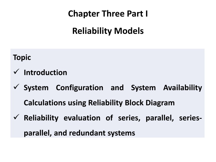
Chapter Three Part I Reliability Models Topic Introduction System Configuration and System Availability Calculations using Reliability Block Diagram Reliability evaluation of series, parallel, series- parallel, and redundant systems

To study reliability, it is necessary to transform reality into a model, which allows the analysis by applying laws and analyzing its behavior Reliability models can be divided into static and dynamic ones. Static models assume that a failure does not result in the occurrence of other faults. Dynamic reliability, instead, assumes that some failures, so- called primary failures, promote the emergence of secondary and tertiary faults, with a cascading effect. In this text we will only deal with static models of reliability.

In the traditional paradigm of static reliability, individual components have a binary status: either working or failed. Systems, in turn, are composed by an integer number n n of components, all mutually independent. Depending on how the components are configured in creating the system and according to the operation or failure of individual components, the system either works or does not work.

Lets consider a generic X system consisting of n elements. The static reliability modeling implies that the operating status of the ith component is represented by the state function Xi defined as: Xi= 1 0 if the ith component works if the ith component fails The state of operation of the system is modeled by the state function (X)= 1 if the system works 0 if the system fails

System Configuration and System Availability Calculations System configurations are often represented graphically with Reliability Block Diagrams (RBDs) where each component is represented by a block and the connections between them express the configuration of the system. System Availability is calculated by modeling the system as an interconnection of parts in series and parallel.

Rules to Decide System Configuration The following rules are used to decide if components should be placed in series or parallel: If failure of a part leads to the combination becoming inoperable, the two parts are considered to be operating in series If failure of a part leads to the other part taking over the operations of the failed part, the two parts are considered to be operating in parallel.

Availability in Series Two parts X and Y are considered to be operating in series if failure of either of the parts results in failure of the combination. The combined system is operational only if both Part X and Part Y are available. From this it follows that the combined availability is a product of the availability of the two parts. The combined availability is shown by the equation on the next slide

Serial reliability

Consider the system in the figure above. Part X and Y are connected in series. The table below shows the availability and downtime for individual components and the series combination. Componentv Availability Downtime X 99% (2-nines) 3.65 days/year Y 99.99% (4-nines) 52 minutes/year X and Y Combined 98.99% 3.69 days/year From the above table it is clear that even though a very high availability Part Y was used, the overall availability of the system was pulled down by the low availability of Part X. A chain is weaker than the weakest link.

Availability in Parallel As stated above, two parts are considered to be operating in parallel if the combination is considered failed when both parts fail. The combined system is operational if either is available. A chain is as strong as the weakest link.

From this it follows that the combined availability is 1 - (both parts are unavailable). The combined availability is shown by the equation below: A = 1-(1-Ax)2

The implications of the above equation are that the combined availability of two components in parallel is always much higher than the availability of its individual components. Consider the system in the figure above. Two instances of Part X are connected in parallel. The table below shows the availability and downtime for individual components and the parallel combination. Component Availability Downtime X 99% (2-nines) 3.65 days/year Two X components operating in parallel 99.99% (4-nines) 52 minutes/year Three X components operating in parallel 99.9999% (6-nines) 31 seconds /year !

From the above table it is clear that even though a very low availability Part X was used, the overall availability of the system is much higher. Thus parallel operation provides a very powerful mechanism for making a highly reliable system from low reliability. For this reason, all mission critical systems are designed with redundant components.

Parallel-Series Reliability State functions for series-parallel systems are obtained by decomposition of the system that are in series or in parallel. The state functions of the subsystems are then combined appropriately, depending on how they are configured. A schematic example is shown in the figure.

Calculation of the state function of a series- parallel. Referring to the configuration of the figure, the state function of the system is calculated by first making the state functions of the parallel of { 1,2} , of { 3,4,5 } and of { 6,7,8,9 } . Then we evaluate the state function of the series of the three groups just obtained.

N-Modular Redundant Systems Redundant system implementations typically use a voting method to determine which are correct. This voting overhead means that true parallel module reliability is typically only approached A system k out of n works if and only if at least k of the n components works. That is, consider a system with N components where the system is considered to be available when at least N-M components are available (i.e. no more than M components can fail). The availability of such a system is denoted by AN,M and is calculated below: Note that a series system can be seen as a system n out of n and a parallel system is a system 1 out of n.

Example Consider a 5 module system requiring 3 correct modules, each with a reliability of 0.95.

Availability Computation Example Understanding the System As a first step, we prepare a detailed block diagram of the system. This system consists of an input transducer which receives the signal and converts it to a data stream suitable for the signal processor. This output is fed to a redundant pair of signal processors.

The active signal processor acts on the input, while the standby signal processor ignores the data from the input transducer. Standby just monitors the sanity of the active signal processor. The output from the two signal processor boards is combined and fed into the output transducer. Again, the active signal processor drives the data lines. The standby keeps the data lines tristated. The output transducer outputs the signal to the external world.

Input and output transducer are passive devices with no microprocessor control. The Signal processor cards run a real-time operating system and signal processing applications. Also note that the system stays completely operational as long as at least one signal processor is in operation. Failure of an input or output transducer leads to complete system failure.

Reliability Modeling of the System The second step is to prepare a reliability model of the system. At this stage we decide the parallel and serial connectivity of the system. The complete reliability model of our example system is shown below:

A few important points to note here are: The signal processor hardware and software have been modeled as two distinct entities. The software and the hardware are operating in series as the signal processor cannot function if the hardware or the software is not operational. The two signal processors (software + hardware) combine together to form the signal processing complex.

Within the signal processing complex, the two signal processing complexes are placed in parallel as the system can function when one of the signal processors fails. The input transducer, the signal processing complex and the output transducer have been placed in series as failure of any of the three parts will lead to complete failure of the system.

Calculating Availability of Individual Components Third step involves computing the availability of individual components. MTBF (Mean time between failure) and MTTR (Mean time to repair) values are estimated for each component For hardware components, MTBF information can be obtained from hardware manufactures data sheets. If the hardware has been developed in house, the hardware group would provide MTBF information for the board.

MTTR estimates for hardware are based on the degree to which the system will be monitored by operators. Here we estimate the hardware MTTR to be around 2 hours. Once MTBF and MTTR are known, the availability of the component can be calculated using the following formula:

Estimating software MTBF is a tricky task. Software MTBF is really the time between subsequent reboots of the software. This interval may be estimated from the defect rate of the system. The estimate can also be based on previous experience with similar systems. Here we estimate the MTBF to be around 4000 hours. The MTTR is the time taken to reboot the failed processor.

Our processor supports automatic reboot, so we estimate the software MTTR to be around 5 minute. Note that 5 minutes might seem to be on the higher side. But MTTR should include the following: Time wasted in activities aborted due to signal processor software crash Time taken to detect signal processor failure Time taken by the failed processor to reboot and come back in service

Component MTBF MTTR Availability Downtime Input Transducer 10.51 minutes/year 100,000 hours 2 hours 99.998% Signal Processor Hardware 10,000 hours 2 hours 99.98% 1.75 hours/year Signal Processor Software 2190 hours 5 minute 99.9962% 20 minutes/year Output Transducer 10.51 minutes/year 100,000 hours 2 hours 99.998%

Things to note from the above table are: Availability of software is higher, even though hardware MTBF is higher. The main reason is that software has a much lower MTTR. In other words, the software does fail often but it recovers quickly, thereby having less impact on system availability. The input and output transducers have fairly high availability, thus fairly high availability can be achieved even without redundant components.

Calculating System Availability The last step involves computing the availability of the entire system. These calculations have been based on serial and parallel availability calculation formulas. Component Availability Downtime Signal Processing Complex (software + hardware) 99.9762% 2.08 hours/year Combined availability of Signal Processing Complex 0 and 1 operating in parallel 99.99999% 3.15 seconds/year Complete System 99.9960% 21.08 minutes/year

Minimal Path Set and the Minimal Cut Set we may use more intricate techniques such as the minimal path set and the minimal cut set, to construct the system state function

Minimal Path Set A Minimal Path Set - MPS is a subset of the components of the system such that the operation of all the components in the subset implies the operation of the system. The set is minimal because the removal of any element from the subset eliminates this property.

The system on the left contains the minimal path set indicated by the arrows and shown in the right part. Each of them represents a minimal subset of the components of the system such that the operation of all the components in the subset implies the operation of the system.

Minimal Cut Set A Minimal Cut Set - MCS is a subset of the components of the system such that the failure of all components in the subset does not imply the operation of the system. Still, the set is called minimal because the removal of any component from the subset clears this property

Minimal Cut Set. The system of the left contains the minimal cut set, indicated by the dashed lines, shown in the right part. Each of them represents a minimum subset of the components of the system such that the failure of all components in the subset does not imply the operation of the system.

MCS and MPS can be used to build equivalent configurations of more complex systems, not referable to the simple series- parallel model. The first equivalent configuration is based on the consideration that the operation of all the components, in at least a MPS, entails the operation of the system. This configuration is, therefore, constructed with the creation of a series subsystem for each path using only the minimum components of that set. Then, these subsystems are connected in parallel.

Equivalent configurations with MPS. You build a series subsystem for each MPS. Then such subsystems are connected in parallel.

Equivalent configurations with MCS. You build a subsystem in parallel for each MCS. Then the subsystems are connected in series.

Examples 1. A serial system consisting of 4 elements with reliability equal to 0.98, 0.99, 0.995 and 0.975. The reliability of the whole system is given by their product: R = 0.98 0.99 0.995 0.975 = 0.941

2. A parallel system consisting of 4 elements with the same reliability of 0.85. The system reliability given by their co-product: 1 - (1 - 0.85)4 = 0.9995.

3. A series-parallel system, drawn below consisting of 9 elements with reliability R1 = R2 = 0.9; R3 = R4 = R5 = 0.8 and R6 = R7 = R8 = R9 = 0.7. Calculate the overall reliability of the system.

For constant per-unit failure rates t = R i ) t ( e i e t = R e i system t = R system = i Per-unit failure rate of series system is constant and equal to the sum of the component failure rates EML4550 -- 2007

For constant per-unit failure rates (example: two systems in parallel) ( 1 e 1 1 + = )( ) t t = R e 1 2 system ( )t + t t R e e e 1 2 1 2 system System does not have constant per-unit failure rate even if components do System reliability for parallel systems is always greater than the most reliable component EML4550 EML4550 -- -- 2007 2007

Most systems are not designed in parallel (redundancy) due to cost considerations (unless needed due to safety and life-protection considerations) Series Transmission line, Power train Parallel Multiple airplane engines, Two headlights

Reliability Marginal Gain Reliability functions of the system can also be used to calculate measures of reliability importance. These measurements are used to assess which components of a system offer the greatest opportunity to improve the overall reliability. The most widely recognized definition of reliability importance I'i of the components is the reliability marginal gain, in terms of overall system rise of functionality, obtained by a marginal increase of the component reliability: