the Method of Auxiliary Sources in Electromagnetic Problems
This presentation by Dr. Assoc. Prof. Vasil Tabatadze introduces the Method of Auxiliary Sources (MAS) theory and its application to electromagnetic problems, focusing on the 2D case and TM field. The theory involves the Helmholtz equation, wave numbers, Hankel functions, and linear integral equations for determining scattered fields in scenarios like perfectly conducting cylinders. It explains the process of satisfying boundary conditions, solving linear algebraic systems, and utilizing scattered field properties to address singularity issues common in other methods.

Download Presentation

Please find below an Image/Link to download the presentation.
The content on the website is provided AS IS for your information and personal use only. It may not be sold, licensed, or shared on other websites without obtaining consent from the author.If you encounter any issues during the download, it is possible that the publisher has removed the file from their server.
You are allowed to download the files provided on this website for personal or commercial use, subject to the condition that they are used lawfully. All files are the property of their respective owners.
The content on the website is provided AS IS for your information and personal use only. It may not be sold, licensed, or shared on other websites without obtaining consent from the author.
E N D
Presentation Transcript
The Method of Auxiliary Sources and its application to the Electromagnetic problems MAS THEORY Presentation by DR. Assoc. Prof. VASIL TABATADZE
TM FIELD j t e Time deppendence is Maxwell equation has the next form = = E j H + H j E J For TM field assume that = ( , ) E u E x y Electric field has only z component z z The same for J. Then Maxwell equations lead to: + = 2 2 E k E j J (1) z z z This is the two-dimensional Helmholtz equation. K is the wave number
k = (2) 0( ' ) E IH k Let s consider field due to the fillament of current I: (2) z 4 = u x u y + Field point radius vector x y = + ' ' ' u x u y source point radius vector x y = / 120 Intrinsic impedance of free space (2) 0 H Hankel function of the second kind and zero order E In (2) is the Green s function of the operator (1) z z E A general solution is then the superposition of Due to all elements of source zJ ds k ( ) = ' (2) 0 ' ' ( ) ( ) E J H k ds z z 4
Main idea of MAS The case of the perfectly conductor cylinder Let s consider cylinder perfectly conductor scatterer with surface C. Incident field excites current on the C and we get the scattered field. In order to find the scattered field we have to determine Currents excited on the surface. For this we have to requre boundary condition sattisfaction on The scatterer s surface. In case of the perfect conductor the tangential component of the total electric field (scattered field + incident field) must be zero. = + = i z s z 0 E E E C z Considering this we get the integral equation: k ( ) = ' (2) 0 ' i z ( ) ( ) E J H k dl C z 4 In order to determine the scattered field we need to find the current distribution first
We represent the scatterer by the discrete N points i We should satisfy the boundary condition sattisfaction in each point.As a result we get linear integral equation system. N k = ' (2) 0 ' i z i ( ) ( ) ( ) E I H k k 1 1 z i i = ' (2) 0 ' i z ( ) ( ) ( ) E J H k dl 4 k = 1 i 1 1 C z 4 k N = ' (2) 0 ' i z i ( ) ( ) ( ) E I H k = ' (2) 0 ' i z ( ) ( ) ( ) E J H k dl 2 2 z i i 4 2 2 C z = 4 1 i . . N k k = ' (2) 0 ' i z i ( ) ( ) ( ) E I H k = ' (2) 0 ' i z ( ) ( ) ( ) E J H k dl N z i N i 4 N C z N 4 = 1 i In order to solve this system we simplify the problem and go from integral to the sum. Instead of continous distribution of current we get discretized current. And instead of linear integral equation system we get linear algebraic system. Each collocation point (where we require boundary condition sattisfaction) corresponds to discrete current point. This gives singularity because of the Hankel s function. Other methods use regularization to avoid singularity (they add a positive number to the green function argument. Some authors requre boundary condition sattisfaction between the points). MAS uses different approach: We use scattered field fundamental property. Scattered field is analytical on the scatterer s surface. Besides the fact that currents are excited on the scatterer surface, the E field value is finite. This is integrable singularity. This gives possibility to analitically continue field inside scatterer. and as a result shift the current surface inside the scatterer so the source points and collocation points does not coincide.
Scatterers and auxiliary surfaces i i We avoid singularity. We solve this system and find the scattered field. N k ( ) = (2) 0 sc z i z i i ( ) ( ) E I H k 4 = 1 i
How to correctly choose the auxiliary surface First it was thought that the auxiliary surface can be at any distance from the real surface. But practice showed that in case of elliptical scatterer when the auxiliary surface occupies ellipse focuses, the series have good convergence but when the auxiliary surface does not occupie the elipse focuses big ammount of the auxiliary sources is neaded that mens that series diverges. converges diverges What is the reason of this?
How to correctly choose the auxiliary surface Let s consider simpler case Image point of the source is the Scattered Field Singularity
In case of the ellipse scattered field singularities coincides to the ellipse focuses for small ka
How to correctly choose the auxiliary surface In case of the circular scatterer field singularities coincides to the caustic surface ka=10 ka=20 scattered field singularities for the ideal conductor cylinder irradiated by the plane wave Auxiliary surface should occupie the scattered field singularity contour. The best case is when auxiliary and scattered field singularity surfaces coinside
Satisfactions of boundary conditions for different removals of auxiliary sources Distance = 0.1m Control points Distance = 0.12m Distance = 0.15m Distance = 0.4m Radius of Sphere is 1m Incident field is dipole. Position= ( 0, 0, 20); Polarization = (0, 1, 0) ; AS Remove makes SF more smooth on the surface and better satisfaction of BC
Advantage 1 of the Method of Auxiliary Sources (MAS) Dependence of the necessary number of terms AS on the relative distance between the auxiliary and boundary surfaces for different precissions of the solution.
Summarize i t e Time dependence: + + = = s s 2 U x y z k U x y z ( , , ) ( , , ) ) 0 Wave equation: Boundary condition: ) x y z S ( , , + + = = s i W U x y z U x y z ( , , ) ( , , , 0 ik r r e n ( 0 ) 1 = = U r H k r r ( ) ( ) U r ( ) 2-D case, 3-D case, n n n r r n = U r j r G ) r r s d ) Metal scatterer ( ) ( ( - Generalized Aux. Source n S n N r r n = s Approximate solution ( , , ) ( ) U x y z j U n n S 1 S root-mean-square error N ~ = n = i ( , , ) ( ) U x y z j U r r n n 1 U s (x,y,z) when tends to exact solution . N s = i ( U ) ( ) U J s kr ds s S Dielectric scatterer
Retarded Hertz Vector Current and charge can be represented with one vector
A multipole expansion This term corresponds to the oscilating electring dipole. The next term is: This correspond to the magnetic dipole and the quadrupole. This term in small and we neglect it.
Field of the dipole We represent the scattered field by the sum of the electric dipole (which is called as Herth dipole) fields. = = + (0) (0) 2 (0) E k j (0) (0) H (1) p In case of the one dipole -is a constant vector and determines the polarisation of the dipole Electric and magnetic fields of the dipole is given by the formulae: (0) R -Is a unit vector directed from the dipole towards the observer and
As in the 2D case the auxiliary surface is shifted. At each point of the auxiliary surface 2 perpendicular electric dipole are located. Boundary conditions are sattisfaied along two perpendicualar tangential vectors 2 -tangential vectors 1,2 r 1 second electric dipole r = sc inc ( )| r ( )| r E E First electric dipole 1 1 = sc inc ( )| r ( )| r E E 2 2 N N = k r + k r sc E E ( ) r ( ) ( ) ( ) ( ) E X r G r X r G r , , i Hertz i Hertz 1 2 = = 1 1 i i
k>0 k<0 N = meas ( ) m r ( ) E A E mn r n aux = + + 2 2 2 ( ) ( ) ( ) mn r x x y y z z = m n m n m n 1 n = 1,... m M Field sof the elementary electric dipoles (k -k ) : = M N 1 i ik R ( ) i t = aux 0 n H R p R , e n 2 n 4 R n ( ) ( ) 2 1 N 1 R ik R k R ( ) ( ) ( ) i t = aux 0 n 0 n 0 n 0 n 0 n 0 n E R R R p p R R p p R R p 3 , 3 , , e n 3 n 2 4 = rec ( ) r ( ) n r E A E = ( , , ) x y z r = + + 2 2 2 ( ) ( ) ( ) r x x y y z z n aux n n n n = 1 n
Scatterer located in vacuum Scatterer could be considered as agregate of surces. Let s consider 3 sources Illuminated source Auxiliary surface Real field Measured surface Reconstructed field
Reconstruction of the field for two sources Real field Reconstructed field K=1


")