Explore the Poisson distribution, named after French mathematician Poisson, commonly used for rare events in large populations. Learn about its approximation to the binomial distribution, assumptions, and calculations. Dive into examples like spina bifida cases and Poisson processes.
Please find below an Image/Link to download the presentation.
The content on the website is provided AS IS for your information and personal use only. It may not be sold, licensed, or shared on other websites without obtaining consent from the author. If you encounter any issues during the download, it is possible that the publisher has removed the file from their server.
You are allowed to download the files provided on this website for personal or commercial use, subject to the condition that they are used lawfully. All files are the property of their respective owners.
The content on the website is provided AS IS for your information and personal use only. It may not be sold, licensed, or shared on other websites without obtaining consent from the author.
E N D
Presentation Transcript
The Poisson Distribution Nina Gunnes January 30, 2019 Lecture 11 1
Poisson distribution https://sco.m.wikipedia.org/wiki/File:Simeon_Poisson.jpg Named after the French mathematician Poisson (1781 1840) Commonly used to describe rare events in a large population Probability distribution: ? ? = ? =??? ? ?: number of cases ?: expected number of cases Expected value equal to the variance E ? = ? = Var ? for ? = 0,1,2, ?! Lecture 11 2
Poisson distribution, cont. Two approaches to the Poisson distribution As an approximation to the binomial distribution Through a Poisson process Lecture 11 4
Approximation to the binomial distribution Binomial distribution approximated by the Poisson distribution ?~Bin ?,? ?~Poi ? Expected number of events: E ? = ? = ?? Two key assumptions for the approximation to be valid Small probability of an event of interest ( success ): ? 0.05 Large number of trials: ? 50 Probability calculations easier with the Poisson distribution Quite demanding using the formula for the binomial distribution Lecture 11 5
Spina bifida (Aalen et al., 2006) Considering a binomial experiment of ? = 5000 births Probability of spina bifida: ? = Number of cases of spina bifida: ? Checking the assumptions for the Poisson approximation ? = 0.001 < 0.05 ? = 5000 > 50 Calculating the expected number of cases of spina bifida ? = ?? = 5000 0.001 = 5 1 1000 Lecture 11 6
Spina bifida (Aalen et al., 2006), cont. Calculating the probability of four cases of spina bifida ? ? = 4 =54? 5 4! = 0.175 = 17.5% Calculating the probability of five cases of spina bifida ? ? = 5 =55? 5 5! = 0.175 = 17.5% Calculating the probability of six cases of spina bifida ? ? = 6 =56? 5 6! = 0.146 = 14.6% Lecture 11 7
Poisson process Objects (or events) distributed randomly over a continuum Time Surface Volume Three fundamental assumptions Expected number of objects per unit (time, surface, volume) being constant Objects appearing randomly and independently of each other No two objects completely coincident in time/space Lecture 11 8
Poisson process, cont. Several examples in real life Childbirths at a maternity ward during a period of time Red blood cells in blood plasma Bacteria in water Implying a Poisson distribution Number of objects (events): ? Expected number of objects (events): ? ?~Poi ? www.publicdomainpictures.net/en/view-image.php?image=127965%26picture=bacteria Lecture 11 9
Anencephaly (Aalen et al., 2006) Considering anencephaly among children who are born A potential increase over time may have different causes Environmental pollutants Radioactivity Medicaments Using data on anencephaly in Edinburgh in 1956 1966 (Osborn, 1979) Number of cases per month 0 1 2 3 4 5 6 7 8 Total Observed number of months 18 42 34 18 11 6 0 2 1 132 Lecture 11 10
Anencephaly (Aalen et al., 2006), cont. Comparing the observed distribution to the Poisson distribution Number of cases per month: ?~Poi ? Estimating the expected number of cases per month ? = 0 18 + 1 42 + 2 34 + + 8 1 Calculating probabilities using the formula for the Poisson distribution ? ? = 0 = 1.970 ? 1.970! = 0.1395 ? ? = 1 = 1.971 ? 1.971! = 0.2748 132 = 260 132 = 1.97 Lecture 11 11
Anencephaly (Aalen et al., 2006), cont. Calculating the expected number of months with 0, 1, 2, etc. cases 0 cases: ? ? = 0 132 = 0.1395 132 = 18.4 1 case: ? ? = 1 132 = 0.2748 132 = 36.3 Number of cases per month 0 1 2 3 4 5 6 7 8 Observed number of months 18 42 34 18 11 6 0 2 1 Expected number of months 18.4 36.3 35.7 23.5 11.5 4.5 1.5 0.4 0.1 Good agreement between observed and expected numbers Lecture 11 12
Malformations (Aalen et al., 2006) Three cases of congenital malformations in B mlo within six months More than what would be expected Investigation carried out to find causes of the overrepresentation Concluded to be the result of coincidence Assuming a Poisson distribution for the number of cases: ?~Poi ? Approximate number of babies born in B mlo during six months: 80 Overall risk of malformations in Norway: 1.6 per 1000 births Expected number of cases in B mlo: ? = 1.6 1000 80 = 0.13 Lecture 11 13
Malformations (Aalen et al., 2006), cont. Calculating probabilities for three or more cases during six months ? ? = 3 = 0.133 ? 0.133! = 0.00032 ? ? = 4 = 0.134 ? 0.134! = 0.00001 ? ? 3 = 0.00032 + 0.00001 + 0.033% Considering 50 municipalities of the same size as B mlo over 5 years 500 six-month periods among all municipalities Probability of at least three cases during six months: 1 1 0.00033500= 0.15 = 15% (not so small anymore!) Lecture 11 14
Lymphoma (Aalen et al., 2006) Considering cases of lymphoma in Seascale in Great Britain Observing increased incidence 4 out of 411 children diagnosed before the age of 15 years Assuming a Poisson distribution for the cases Number of cases: ? Expected number of cases (based on data from around the district): ? = 0.25 ?~Poi ? Excess of cases due to the nuclear power plant in Windscale? Lecture 11 15
Lymphoma (Aalen et al., 2006), cont. Defining the hypotheses for a one-sided test Null hypothesis, ?0: ? = 0.25 One-sided alternative hypothesis, ??: ? > 0.25 Choosing a significance level of 1% Evidence must be compelling before rejecting the null hypothesis Calculating the p value ? ? 4|? = 0.25 0.254 ? 0.254! + Rejecting the null hypothesis and claiming increased risk of lymphoma 0.255 ? 0.255! = 0.00014 Lecture 11 16
Normal approximation to Poisson Poisson distribution resembling a normal distribution when ? is large Expected value (mean) of ?: E ? = ? Variance of ?: Var ? = ? Standard deviation of ?: SD ? = Using ? = 5 as a lower limit for the approximation The larger ?, the better the approximation Poor approximation when ? < 5 The two distributions coinciding when ? ? http://www.thescientificcartoonist.com/?paged=109 Lecture 11 17
Death in traffic (Aalen et al., 2006) Considering traffic deaths among people aged 15 24 years Approximately 120 persons killed in traffic each year for several years Assuming a Poisson distribution Number of persons killed: ? Expected number of persons killed: ? ?~Poi ? Imagining the number of persons killed being reduced to 90 one year Coincidence or an indication of a real risk reduction? Lecture 11 19
Death in traffic (Aalen et al., 2006), cont. Defining hypotheses for a two-sided test Null hypothesis, ?0: ? = 120 Two-sided alternative hypothesis, ??: ? 120 Choosing a significance level of 5% Defining the p value: ? ? 90 or ? 150|?0 Probability of a result at least as extreme as that observed in either direction Using the normal approximation under the null hypothesis ?~N 120, 120 Lecture 11 20
Death in traffic (Aalen et al., 2006), cont. Calculating the p value by standardizing ? ? 90 + ? ? 150 = 2 ? ? 90 = 2 ? 2 ? ? 2.74 = 2 0.0031 = 0.0062 = 0.62% Rejecting the null hypothesis based on the p value Real reduction in risk of being killed in traffic More exact result by using continuity correction Improving the normal approximation Calculating 2 ? ? 90.5 instead of 2 ? ? 90 ? 120 120 90 120 120 Lecture 11 21
Comparison of two Poisson variables Considering two independent Poisson distributed variables Numbers of cases: ?1and ?2 Expected values: ?1and ?2 Do the expected values differ? Null hypothesis, ?0: ?1= ?2 Test statistic: ? = ?1 ?2 Follows a standard normal distribution, i.e., ?~N 0,1 ?1+ ?2 Lecture 11 23
Traffic fatalities (Aalen et al., 2006) Considering traffic fatalities over two years First year: ?1= 338 Second year: ?2= 401 Expected values: ?1and ?2 Real change in risk or just a coincidence? Defining the hypothesis for a two-sided test Null hypothesis, ?0: ?1= ?2 Two-sided alternative hypothesis, ??: ?1 ?2 Lecture 11 24
Traffic fatalities (Aalen et al., 2006), cont. Choosing a significance level of 5% Calculating the observed value of the test statistic ?obs= 338 401 Calculating the p value 2 ? ? 2.32 = 2 0.0102 = 2% Rejecting the null hypothesis based on the p value The observed increase in traffic fatalities indicating a real change 338 + 401 = 2.32 Lecture 11 25
References Aalen OO, Frigessi A, Moger TA, Scheel I, Skovlund E, Veier d MB. 2006. Statistiske metoder i medisin og helsefag. Oslo: Gyldendal akademisk. Lecture 11 26


")
, cont.")


")
, cont.")
, cont.")
")
, cont.")
")
, cont.")


")
, cont.")
, cont.")
, cont.")

")
, cont.")