The Science of Statistics: Descriptive vs. Inferential, Variables, Data Types & More

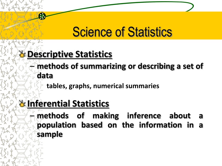
Science of Statistics Descriptive Statistics methods of summarizing or describing a set of data tables, graphs, numerical summaries Inferential Statistics methods population based on the information in a sample of making inference about a

Variables Individuals are the objects described by a set of data; may be people, animals or things Variable is any characteristic of an individual

Statistical Data What purpose do the data have? Individuals Describe? How many? Variables How many? Definition? measurement? Unit of

Types of Variables Categorical variable places an individual into one of several groups or categories Quantitative variable takes numerical values for which arithmetic operations make sense Distribution of a variable tells us what values it takes and how often it takes these values

Exploratory Data Analysis Examine relationships among the variables each variable by itself then Start summaries of specific aspects of the data with graphs then add numerical

Levels of Measurement Nominal Ordinal Interval Ratio It's hierarchy implied in the level of measurement idea. At each level up the hierarchy, the current level includes all of the qualities of the one below it and adds something new. In general, it is desirable to have a higher level of measurement. important to recognize that there is a

In nominal measurement the numerical values just "name" the attribute uniquely. No ordering of the cases is implied. For example, jersey numbers in basketball are measures at the nominal level. Is a player with number 30 more of anything than a player with number 15?

In ordinal measurement the attributes can be rank- ordered. Here, distances between attributes do not have any meaning. For example, on a survey you might code Educational Attainment as 0=less than H.S.; 1=some H.S.; 2=H.S. degree; 3=some college; 4=college degree; 5=post college. In this measure, higher numbers mean more education. But is distance from 0 to 1 same as 3 to 4?

In interval measurement the distance between attributes does have meaning. For example, when we measure temperature (in Fahrenheit), the distance from 30-40 is same as distance from 70-80. The interval between values is interpretable. Because of this, it makes sense to compute an average of an interval variable, where it doesn't make sense to do so for ordinal scales. Do ratios make sense at this level? For example, is it twice as hot at 80 degrees as it is at 40 degrees?

Finally, in ratio measurement there is always an absolute zero that is meaningful. This means that you can construct a meaningful ratio. Weight is a ratio variable. In applied social research most "count" variables are ratio. Is number of clients in past six months ratio? Why?

Describing Graphically Bar Graph: count or percent Pie Chart: parts of the whole Stem Plot: shape of distribution Histogram: great when lots of groups Frequency Table

Time Plots Time Series: measurements of a variable taken at regular intervals over time Residual Plots: checking assumptions Trends, such as seasonal variation

Outliers Extreme Values What do you do with outliers? Ignore them Throw them out ?

Graphical Examples Let s Take a Look

Choosing a Summary The five-number summary is usually better than the mean and standard deviation for describing a skewed distribution or a distribution with strong outliers. Use the mean and standard deviation for reasonably symmetric distributions that are free of outliers.

Describing Distributions with Numbers Mean: simple average is sensitive to extreme scores not necessarily a possible value To calculate: add the values and divide by the number of items

Median: middle score not sensitive to extreme scores To Calculate: rank data from smallest to largest if n is odd, median is the middle score if n is even, median is the average of two middle scores

Mode: most frequent score does not always exist unstable can be used with qualitative data

Measures of Dispersion (Variability) Range totally sensitive to extreme scores easy to compute To Calculate: high score low score

Variance Variance: measures squared distances from the mean large values of suggest large variability Standard Deviation: square root of the variance

Empirical Rule Should be used for moundshape data approx. 68% of the data fall between mean +/- SD approx. 95% of the data fall between mean +/- 2 * SD approx. 99.7% of the data fall between mean +/- 3 * SD

Lets give it a try Let s use faculty experience. Why? What should we do with it?

Quartiles and 5-Number Summary Quartiles divide ordered numerical data into four equally sized parts. 1st quartile, Q1, 25% below and 75% above 2nd quartile, Q2, median, 50% below and 50% above 3rd quartile, Q3, 75% below and 25% above The low score, Q1, Q2, Q3, and the high score are known as the five number summary of a data set.

BoxPlots Particularly helpful in comparing 2 or more groups Box shows central 50% of data and the median Whiskers show extremes

Lets give it a try Let s use the $ in the pocket data. Why? What should we do with it?

1.5 X IQR Criterion Interquartile Range is the distance between the 1st and 3rd quartiles Call an observation a suspected outlier if it falls more than 1.5 X IQR above the 3rd quartile or below the 1st quartile Example on page 46

Normal Distributions Density Curve: can often describe the overall pattern of a distribution Total area of 1 under the curve Areas under the curve are relative frequencies The mean, median, and quartiles can be eyed on a density curve.

Normal Distributions Bell-shaped, symmetric, unimodal curve The mean and standard deviation completely specify the normal distribution N ( ) , Mean is the center of symmetry SD is the distance from the mean to the change of curvature points

Standardizing Observations The Z-score of an observation gives the # of standard deviations it is above or below the mean x x x = z s

Standard Normal Standard Normal is a special case of the normal where N(0,1) Let s We will need to use Table A. do some examples.