Time-Frequency Analysis Methods and Applications: Joint Distribution Reference

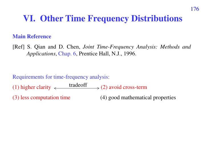
176 VI. Other Time Frequency Distributions Main Reference [Ref] S. Qian and D. Chen, Joint Time-Frequency Analysis: Methods and Applications, Chap. 6, Prentice Hall, N.J., 1996. Requirements for time-frequency analysis: tradeoff (1) higher clarity (2) avoid cross-term (3) less computation time (4) good mathematical properties

177 VI-A Cohen s Class Distribution VI-A-1 Ambiguity Function ( ) ( ) ( ) = + x t * 2 j t , / 2 / 2 x A x t e dt ( ) x t = + 2 exp ( ) 2 t t j f t (1) If 0 0 ( ) 2 2 + + + ( /2 ) 2 ( /2) ( /2 ) 2 ( /2) = t t j f t t t j f t 2 j t , A e e e dt 0 0 0 0 x 2 2 t t + + 2( ) /2 2 j f = 2 j t e e dt 0 0 2 2 + + 2 /2 2 t j f 2 = j t 2 j t e e e dt 0 0 2 2 1 ( ) ( ) = + 0 , exp exp 2 x A j f t 0 2 2 2

178 WDF and AF for the signal with only 1 term AF WDF f ( ) , t f 0 0 t

179 ( ) x t = + + + 2 2 exp ( ) 2 exp ( ) 2 t t j f t t t j f t (2) If 1 1 1 2 2 2 x1(t) x2(t) ( ) ( ) ( ) ( ) x A , = + x t + 2 j t , / 2 / 2 A x t e dt 1 1 x 1 ( ) ( ) ( ) , x A + x t + 2 j t / 2 / 2 x t e dt 2 2 2 ( ) ( ) ( ) , A + x t + 2 j t / 2 / 2 x t e dt 1 2 x x 1 2 ( ) ( ) ( ) , A + x t + 2 j t / 2 / 2 x t e dt 2 1 x x 2 1 ( ) ( ) ( ) ( ) ( ) = + + + , , , , , A A A A A x x x 1 2 x x 2 1 x x 1 2 2 2 1 ( ) ( ) = + 1 , exp exp 2 1 2 x A j f t 1 2 2 1 1 1 2 2 1 ( ) ( ) = + 2 , exp exp 2 2 2 x A j f t 2 2 2 2 2 2

180 When 1= 2 ( 2 2 ( ) ) t f 1 ( ) = + , exp d d A 2 2 2 1 2 x x 2 ( + exp ) j f t f t d = = + = = + = + ( )/2, ( )/2, ( = )/2, t t t f f f 1 2 1 2 1 2 , , t t t f f f 1 2 1 2 1 2 d d d ( ) ( ) = , , A A 2 1 x x 1 2 x x When 1 2 + + 2 [( ) ( ) / 2] f j 1 1 t 2 2 t j 1 ( ) = , exp d d A 2 2 1 2 x x ) ( + + 2 2 exp ( ) ( ) exp 2 t t j f 1 1 2 2 2 2 ( ) ( ) = , , A A 2 1 x x 1 2 x x

181 WDF and AF for the signal with 2 terms f auto term |WDF| (t1, f1) cross terms (t , f ) t (t2, f2) |AF| cross term auto term (td , fd) auto terms (0, 0) cross term (-td , -fd)

182 For the ambiguity function The auto term is always near to the origin The cross-term is always far from the origin

183 VI-A-2 Definition of Cohen s Class Distribution The Cohen s Class distribution is a further generalization of the Wigner distribution function ( ) ( ) ( , , x x C t f A ) ( ) = 2 ( d d , exp ) j t f ( ) ( ) ( ) = + x t * 2 j t , / 2 / 2 x A x t e dt where is the ambiguity function (AF). ( , ) = 1 WDF ( x C t f ) ( ) ( ) ( ) = + * 2 j f , /2 /2 , x u x u t u du e d ( ) ( ) = where , , exp( 2 ) t j t d

184 How does the Cohen s class distribution avoid the cross term? Chose ( , ) low pass function. ( , ) 1 for small | |, | | ( , ) 0 for large | |, | | [Ref] L. Cohen, Generalized phase-space distribution functions, J. Math. Phys., vol. 7, pp. 781-806, 1966. [Ref] L. Cohen, Time-Frequency Analysis, Prentice-Hall, New York, 1995.

185 VI-A-3 Several Types of Cohen s Class Distribution Choi-Williams Distribution (One of the Cohen s class distribution) ( ) ( ) 2 = , exp [Ref] H. Choi and W. J. Williams, Improved time-frequency representation of multicomponent signals using exponential kernels, IEEE. Trans. Acoustics, Speech, Signal Processing, vol. 37, no. 6, pp. 862-871, June 1989.

186 Cone-Shape Distribution (One of the Cohen s class distribution) ) ( ) ( t 1 ( ) = 2 , exp 2 t | | ( ) ( ) ( ) = 2 , sin exp 2 c [Ref] Y. Zhao, L. E. Atlas, and R. J. Marks, The use of cone-shape kernels for generalized time-frequency representations of nonstationary signals, IEEE Trans. Acoustics, Speech, Signal Processing, vol. 38, no. 7, pp. 1084-1091, July 1990.

187 Cone-Shape distribution for the example on pages 96, 149 ( = 1) 4 3 2 1 frequency 0 -1 -2 -3 -4 -8 -6 -4 -2 0 2 4 6 8 time (sec)

188 ( , ) Distributions Wigner 1 ( , ) = 1 for ( , ) = 0 otherwise ( , ) = 1 for ( , ) = 0 otherwise Cohen (circular) + 2 2 r Cohen (rectangular) ( , ) Max T Choi-Williams ( ) ) 2 exp Cone-Shape ( ) ( c ) 2 sin exp ( ( 2 Page exp j ) cos Levin (Margenau-Hill) ( ) sinc Born-Jordan 2007

189 VI-A-4 Advantages and Disadvantages of Cohen s Class Distributions The Cohen s class distribution may avoid the cross term and has higher clarity. However, it requires more computation time and lacks of well mathematical properties. Moreover, there is a tradeoff between the quality of the auto term and the ability of removing the cross terms.

190 VI-A-5 Implementation for the Cohen s Class Distribution ( ) ( ) ( + ) ( ) = 2 ( d d , , , exp ) C t f A j t f x x ) ( ) ( ( ) + 2 ( = * 2 ) j u j t f , x u x u e dud d 2 2 1 Ax( , ) If for | | > B or | | > C ( ) , 0 = ) ( ) ( C B ( ) ( ) + 2 ( = + * 2 ) j u j t f , , C t f x u x u e dud d x 2 2 C B

191 2 input output ) ( ) ( ) ) ( ( C B ( ) ( ) t u = + * 2 ( ) 2 j j f , [ , ] C t f x u x u e d e dud x 2 2 C B C ( ) = + * 2 j f , x u x u t u e dud 2 2 C B ( ) ( ) = 2 j t , , t e d B input 2 ( ) ,t

192 VI-B Modified Wigner Distribution Function ( ) ( ) ( ) = + x t * 2 j f , / 2 / 2 W t f x t e d x ( ) ( ) = + X * 2 j t / 2 / 2 X f f e d where X(f) = FT[x(t)] Modified Form I B ( ) ( ) ( ) ( ) = + x t * 2 j f , / 2 / 2 W t f w x t e d x B Modified Form II B ( ) ( ) ( ) ( ) = + X * 2 j t , / 2 / 2 W t f w X f f e d x B

193 Modified Form III (Pseudo L-Wigner Distribution) ) ) ( ) ( ( ( ) = + 2 L L j f , W t f w x t x t e d 2 2 x L L L cross term ( ) [Ref] L. J. Stankovic, S. Stankovic, and E. Fakultet, An analysis of instantaneous frequency representation using time frequency distributions-generalized Wigner distribution, IEEE Trans. on Signal Processing, pp. 549-552, vol. 43, no. 2, Feb. 1995 P.S.: 2006

194 Modified Form IV (Polynomial Wigner Distribution Function) /2 q ( ) = + l l 2 j f , ( ) ( ) W t f x t d x t d e d x = 1 l When q = 2 and d1= d-1= 0.5, it becomes the original Wigner distribution function. It can avoid the cross term when the order of phase of the exponential function is no larger than q/2 + 1. However, the cross term between two components cannot be removed. [Ref] B. Boashash and P. O Shea, Polynomial Wigner-Ville distributions & their relationship to time-varying higher order spectra, IEEE Trans. Signal Processing, vol. 42, pp. 216 220, Jan. 1994. [Ref] J. J. Ding, S. C. Pei, and Y. F. Chang, Generalized polynomial Wigner spectrogram for high-resolution time-frequency analysis, APSIPA ASC, Kaohsiung, Taiwan, Oct. 2013.

195 dlshould be chosen properly such that /2 1 + /2 q q + l l = 1 n ( ) ( ) ex p 2 x t d x t d j na t n = = 1 n 1 l /2 1 + q ( ) t = n when exp 2 x j a t n = 1 n then /2 1 + /2 1 + q q ( ) = 2 ( 1 1 n n , exp ) W t f j f na t d f na t x n n = = 1 1 n n (from page 138(1)) page 138(3)

196 /2 1 + /2 q q + l l = 1 n ( ) ( ) ex p 2 x t d x t d j na t n = = 1 n 1 l /2 1 + q ( ) t = n exp 2 x j a t n = 1 n ( ) ( ) x t = 2 ( + 2 when q = 2 exp ) j at a t 1 2 ( ) + 1 1 = 2 ( + ( ) ( ) exp 2 ) x t d x t d j a a t 1 2 ( ) ( ) ( ) ( ) 2 2 + 1 + + 1 1 1 = + 1 2 a t d a t d a t d a t d a t a 2 1 2 1 2 + + + + = + 1 2 2 2 2 ( ) ( ) ( ) 2 a d d t a d d a d d a t a 2 1 1 2 1 1 1 1 1 2 + = = 1 0 d d d d 1 1 1 1 = = 1/ 2 d d 1 1

197 ( ) ( ) x t = 2 ( + + 2 3 exp ) j at a t a t When q = 4, 1 2 3 2 3 + l l = 1 n ( ) ( ) e p x 2 x t d x t d j na t n = = 1 n 1 l 3 + 1 1 + = 1 n ( ) ( ) ( x t ) ( ) exp 2 x t d x t d d x t d j na t 2 2 n = 1 n ( ) ( ) ( ) 3 2 + 1 + + 1 + + 1 a t d a t d a t d 3 2 1 ( ( ( ) ( ) ( ) 3 2 + + + + + + a t d a t d a t d 3 2 2 2 1 2 ) ) ( ( ) ) ( ( ) ) 3 2 1 1 1 a t d a t d a t d 3 2 1 3 2 a t d a t d a t d 3 a t 2 2 2 a 2 1 2 = + + 2 3 a t 3 2 1 + + + = 1 d d d d 1 2 1 2 + = 2 2 2 2 2 0 d d d d 1 1 2 + + + = 3 1 3 2 3 3 0 d d d d 1 2

198 = 5 ( 4 2 ( ) x t exp( ( 5) 5) ) j t j t q = ?

199 = + 3 ( ) x t 2cos(( 5) 4 ) t t

200 VI-C Gabor-Wigner Transform [Ref] S. C. Pei and J. J. Ding, Relations between Gabor transforms and fractional Fourier transforms and their applications for signal processing, IEEE Trans. Signal Processing, vol. 55, no. 10, pp. 4839-4850, Oct. 2007. Advantages: combine the advantage of the WDF and the Gabor transform advantage of the WDF higher clarity advantage of the Gabor transform no cross-term

201 ( ) = 2 x , ( , ) ( , ) D t f G t f W t f x x x(t) = cos(2 t) (b) (a) x(t) Gabor 1 5 0.5 0 0 -0.5 -5 -1 0 2 4 6 8 10 0 2 4 6 8 10 (d) (c) WDF Gabor-Wigner 5 5 0 0 -5 -5 0 2 4 6 8 10 0 2 4 6 8 10

( ) ( ) = ( ) 202 = 2 = , min | ( , )| ,| G t f ( , )| D t W t f , ( , ) ( , ) D t f ( x D t f G t f W t f (a) (b) x x x x x x ) , ( , ) | ( , )| 0.25 G t f (c) W t f x x (d) ( ) , x x D t f G = 2.6 0.7 x ( , ) t f W ( , ) t f (a) (b) 4 4 2 2 f-axis f-axis 0 0 -2 -2 -4 -4 -5 0 5 -5 0 5 (b) (c) are real t-axis (c) t-axis (d) 4 4 2 2 f-axis f-axis 0 0 -2 -2 -4 -4 -5 0 5 -5 0 5 t-axis t-axis

203 (1) Which type of the Gabor-Wigner transform is better? (2) Can we further generalize the results?

204 Implementation of the Gabor-Wigner Transform ( ) = , ( , ) t f W ( , ) t f 0 (1) When Gx(t, f) 0, D t f G x x x Gx(t, f) Wx(t, f) Gx(t, f) 0 (2) When x(t) is real Gabor transform = ( ) ( ) X f X f if x(t) is real, where X(f) = FT[x(t)]

205 Properties of the Fourier Transform ( ) ( ) ( ) x t ( ) = = f t dt exp 2 X f FT x t j (1) Recovery (inverse Fourier transform) ( ) x t ( ) ( ) = f t df exp 2 X f j ( ) 0 ( ) = x X f df (2) Integration ( ) ( ) FT x t e = 2 j f t X f f 0 (3) Modulation 0 ( ) ( ) 2 = j f t FT x t t X f e 0 (4) Time Shifting 0 f a ) 1 a ( ) = FT x at X (5) Scaling | | ( ) ( = FT x t X f (6) Time Reverse If , then X(f) is real. ( ) ( ) x t x t = (7) Real Output

206 If x(t) is real, then X(f) = X*( f); If x(t) is pure imaginary, then X(f) = X*( f) (8) Real / Imaginary Input If x(t) = x( t), then X(f) = X( f); If x(t) = x( t), then X(f) = X( f); (9) Even / Odd Input ( ) ( ) FT x t = X f (10) Conjugation ( ) ( ) (11) Differentiation = f X f 2 FT x t j j ( ) ( ) f = (12) Multiplication by t FT tx t X 2 ( ) x t t = f ( ) 2 (13) Division by t FT j X d (14) Parseval s Theorem (Energy Preservation) ( ) x t ( ) 2 2 = dt X f df ( ) x t y t dt ( ) ( ) ( ) f df (15) Generalized Parseval s Theorem = X f Y

207 ( ) ( ) ( ) ( ) + = + (16) Linearity FT ax t by t aX f bY f ( ) z t ( ) x t ( ) ( ) ( ) = ( ) Z f = , y t ( ) ( ) X f Y f x y t d If (17) Convolution = then If , then ( ) ( ) ( ) z t x t y t = ( ) ( ) Z f X f = ( ) Z f = (18) Multiplication ( ) ( ) ( ) = Y f X Y f d ( ) z t ( ) ( ) X f Y ( ) = , x y t d If (19) Correlation ( ) f then (20) Two Times of Fourier Transforms ( ) ( ) = FT FT x t x t ( ) (21) Four Times of Fourier Transforms ( ) ( ) x t FT FT FT FT x t =