Time-Frequency Analysis: Motions and Transformations Overview

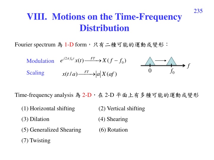
235 VIII. Motions on the Time-Frequency Distribution Fourier spectrum 1-D form 2 j f t FT ( ) x t ( ) e X f f Modulation 0 0 f 0 f0 Scaling FT ( / ) x t a ( ) a X af Time-frequency analysis 2-D 2-D (1) Horizontal shifting (2) Vertical shifting (3) Dilation (4) Shearing (5) Generalized Shearing (6) Rotation (7) Twisting

236 8-1 Basic Motions (1) Horizontal Shifting ( x t t 2 j f t ) ( ( x , ) , ) ,Wigner f ,STFT, Gabor S t W t t f e 0 0 0 t x 0 (2) Vertical Shifting 2 j f t ( ) x t ( , ( , x ) ,STFT,Gabor ) ,Wigner e S t f W t f f 0 0 x f 0

237 (3) Dilation (scaling) 1 | | a t t f ( ) a ( , a ) ,STFT,Gabor x S af x t t ( , a ) ,WDF W af x

238 (4) Shearing 2 t j 2 j at = = ( ) x t ( ) y t ( ) x t ( ) y t e e a f 2 j at = ( ) ( , ) x S t f W t f ( ) ( , x t e y t = ) ,STFT,Gabor S t f at y t ( , ) ( , ) ,WDF W t f at x y 2 t j = ( ) ( , ) x S t f W t f ( ) ( means convolution) , ) , STFT,Gabor af f x t e y t a = ( S t y ( , ) ( , ) , WDF af f W t x y

239 2 j at (Proof): When = ( ) x t ( ), y t e ( ) ( ) ( ) = + * 2 j f , /2 /2 W t f x t x t e d x ( ) ( ) ( ) ( ) 2 2 j a t + j a t /2 /2 = + * 2 j f /2 /2 e e y t y t e d ( ) ( ) = + 2 * 2 j at j f /2 /2 e y t y t e d ( ) ( ) f at = + * 2 ( ) j /2 /2 y t y t e d ( ) = , W t f at y

240 (5) Generalized Shearing ( ) t j = ? ( ) x t ( ) y t e n = k ( ) t a t k = 0 k ( , ) S t f ( , ) ,STFT,Gabor S t f x y ( , ) ( , ) ,WDF W t f W t f x y J. J. Ding, S. C. Pei, and T. Y. Ko, Higher order modulation and the efficient sampling algorithm for time variant signal, European Signal Processing Conference, pp. 2143-2147, Bucharest, Romania,Aug. 2012. J. J. Ding and C. H. Lee, Noise removing for time-variant vocal signal by generalized modulation, APSIPA ASC, pp. 1-10, Kaohsiung, Taiwan, Oct. 2013

241 Q: n = = k If where ( ) x t ( ) ( ) y t ( ) exp h t h t IFT j a f k = 0 k then n 1 + 1 k ( , ) S t f ( , ) ,STFT,Gabor S t ka f f x y k 2 = 1 n k 1 + 1 k ( , ) ( , ) ,WDF W t f W t ka f f x y k 2 = 1 k

242 8-2 Rotation by /2: Fourier Transform = ( ) ( , )| | X t f t f t f ( ( )) S X f S FT x t = = | ( , )| ,STFT f t x 2 j ft ( , ) ( , ) ( ( , ) , ) ,WDF f t ,Gabor G W G W f t e X x X x (clockwise rotation by 90 ) Strictly speaking, the rec-STFT have no rotation property.

243 For Gabor transforms, if ( ) , x G t f ( ) = 2 , ( ) 2 t j f e e x d ( ) ( ) ( ) ( ) x t e = = 2 = ( ) 2 2 t j f j f t , ( ) G t f e e X d X f FT x t dt X ) ( ( ) then = 2 j t f , , G t f G f t e X x (clockwise rotation by 90 for amplitude) ( ) , X G t f e ( ) x u e ( )( Since ( ( ) x u e ) ) ( = 2 ( ( ) 2 2 t j f j u e dud (Proof): = 2 f u + ( ) 2 ( ) t j e d du ( ) 2 ( ) x u 2 2 + = = ( ) 2 ( ) ( ) t j f u t x u e e d du FT e du + f f u ) ) 2 2 2 2 = = ( ) f t j tf f , FT e e FT e e e ( ) ( ) x u e 2 t f u + + = 2 ( ) ( ) j f u , G t f e du X ( ) x u e ( ) 2 = = 2 2 ( ( )) 2 j tf j tu u f j t f , e e du G f t e x

244 If we define the Gabor transform as ( ) , x G t f e = , ( ) 2 ( ) 2 j f t t j f e e x d ( ) ( ) 2 = ( ) 2 j f t t j f , and G t f e e e X d X ( ) ( ) = , , G t f G f t then X x

245 ( ) ( ) ( ) = + x t * 2 j f , /2 /2 W t f x t e d If is the WDF of x(t), x ( ) ( ) ( ) = + X * 2 j f , /2 /2 W t f X t t e d is the WDF of X( f ), X ( ) ( ) then = , , W t f W f t X x (clockwise rotation by 90 ) time-frequency distribution

246 If ( ) X f ( ) x t e = ) t , then = 2 j f t ( ) IFT x t dt ( ) ( , ( ) ( ) = = t e 2 j t f , , W t f W f , , G t f G f X x X x (counterclockwise rotation by 90 ). ( ) ( ) = If X f x t , then ( ) ( ) = ( ) ( ) , , G t f G t f , . = , , W t f W t f X x X x (rotation by 180 ).

247 Examples: x(t) = (t), X(f) = FT[x(t)] = sinc( f ). WDF of (t) WDF of sinc( t ) 2 2 1 1 0 0 -1 -1 -2 -2 -2 -1 0 1 2 -2 -1 0 1 2 Gabor transform of (t) Gabor transform of sinc( t ) 3 3 2 2 1 1 0 0 -1 -1 -2 -2 -3 -3 -3 -2 -1 0 1 2 3 -3 -2 -1 0 1 2 3

248 If a function is an eigenfunction of the Fourier transform, ( ) x t dt ( ) x f = 2 j f t = 1, j, 1, j e then its WDF and Gabor transform have the property of ( ) ( ) , , x x W t f W f t = ( ) ( ) = , , G t f G f t x x ( 90 Example: Gaussian function ( ) 2 exp t

249 Hermite-Gaussian function ( ) ( ) t ( ) t = 2 exp t H m m m d dt ( ) t ( ) t ( ) t 2 2 = 2 2 t t H C e e Hermite polynomials: , Cmis some constant, m m m ( ) ( ) ( ) = 2 H t = = 4 1 H t 1 H t t 2 0 1 = = + 3 2 4 2 4 3 16 24 3 H t t t H t t 3 4 ( ) t H ( ) t 2 , Dmis some constant, = 2 t e H D , m n m m n m,n= 1 when m = n, m,n= 0 otherwise. [Ref] M. R. Spiegel, Mathematical Handbook of Formulas and Tables, McGraw-Hill, 1990.

250 Hermite-Gaussian functions are eigenfunctions of the Fourier transform ( ) t e ( ) ( ) f m = 2 j f t dt j m m Any eigenfunction of the Fourier transform can be expressed as the form of = ( ) ( ) t k t a where r = 0, 1, 2, or 3, a4q+rare some constants ( ) k f q r + q r + 4 4 = 0 q ( ) ( ) r = 2 j f t k t e dt j

251 WDF for 1(t) Gabor transform for 1(t) 3 2 2 1 1 0 0 -1 -1 -2 -3 -2 -3 -2 -1 0 1 2 3 -2 -1 0 1 2 WDF for 2(t) Gabor transform for 2(t) 2 3 2 1 1 0 0 -1 -1 -2 -2 -3 -2 -1 0 1 2 -3 -2 -1 0 1 2 3

252 Problem: How to rotate the time-frequency distribution by the angle other than /2, , and 3 /2?

253 8-3 Rotation: Fractional Fourier Transforms (FRFTs) ( ) x t dt e e e 2 csc cot ( ) u u 2 j j t t 2 u = cot j 1 cot X j , = 0.5a When = 0.5 , the FRFT becomes the FT. Additivity property: ( ) u If we denote the FRFT as (i.e., ) F O ( ) ( ) F F F O O x t O x t = = ( ) x t X O F + then Physical meaning: Performing the FT a times.

254 cot cot 2 1 cot j ( ) x t dt 2 j t u e e e j ( ) u u csc j t = 2 X 2 Another definition 2 [Ref] H. M. Ozaktas, Z. Zalevsky, and M. A. Kutay, The Fractional Fourier Transform with Applications in Optics and Signal Processing, New York, John Wiley & Sons, 2000. [Ref] N. Wiener, Hermitian polynomials and Fourier analysis, Journal of Mathematics Physics MIT, vol. 18, pp. 70-73, 1929. [Ref] V. Namias, The fractional order Fourier transform and its application to quantum mechanics, J. Inst. Maths. Applics., vol. 25, pp. 241-265, 1980. [Ref] L. B. Almeida, The fractional Fourier transform and time-frequency representations, IEEE Trans. Signal Processing, vol. 42, no. 11, pp. 3084-3091, Nov. 1994. [Ref] S. C. Pei and J. J. Ding, Closed form discrete fractional and affine Fourier transforms, IEEE Trans. Signal Processing, vol. 48, no. 5, pp. 1338-1353, May 2000.

255 ( ( ) ( ) = ( ) = FT x t X f ( ) ( ) ) ( ) FT FT x t FT FT FT x t x t = ( ) ) ( ) = X f IFT f t ( ( ) x t FT FT FT FT x t = What happen if we do the FT non-integer times? Physical Meaning: Fourier Transform: time domain frequency domain Fractional Fourier transform: time domain fractional domain Fractional domain: the domain between time and frequency (partially like time and partially like frequency)

256 Experiment: 2 2 2 = = = f(t): rectangle 1 1 1 0 0 0 -1 -1 -1 -5 0 5 -5 0 5 -5 0 5 2 2 2 = = = 1 1 1 0 0 0 F(w): sinc function -1 -1 -1 -5 0 5 -5 blue line: real part green line: imaginary part 0 5 -5 0 5 [Ref] L. B. Almeida, The fractional Fourier transform and time-frequency representations, IEEE Trans. Signal Processing, vol. 42, no. 11, pp. 3084-3091, Nov. 1994.

257 Time domain Frequency domain fractional domain Modulation Shifting Modulation + Shifting Shifting Modulation Modulation + Shifting Differentiation j2 f Differentiation and j2 f j2 f Differentiation Differentiation and j2 f ( ) ( ) ( ) FT exp 2 x t t j ft X f 0 0 ( ) ( ) ( ) fractional FT exp 2 sin cos x t t j j ut X u t 0 0 0 = 2 0sin cos t dx t dt ( ) ( ) f X f FT 2 j d dt d du ( ) x t ( ) ( ) fractional FT u X u + 2 sin cos j X u

258 [Theorem] The fractional Fourier transform (FRFT) with angle is equivalent to the clockwise rotation operation with angle for the Wigner distribution function (or for the Gabor transform) FRFT with parameter = with angle For the WDF If Wx(t, f ) is the WDF of x(t), and WX (u, v) is the WDF of X (u), (X (u) is the FRFT of x(t)), then ( ) ( ) = sin , sin + , cos cos W u v W u v u v X x

259 For the Gabor transform (with standard definition) If Gx(t, f ) is the Gabor transform of x(t), and GX (u, v) is the Gabor transform of X (u), then ( ) , X G u v e ( ) 2 2 2 [ 2 + )sin(2 )/2] = sin , sin + sin ( j uv u v cos cos G u v u v x ( ) ( ) = sin , sin + , cos cos G u v G u v u v X x For the Gabor transform (with another definition on page 244) ( ) ( , cos sin , sin X x G u v G u v ) = + cos u v The Cohen s class distribution and the Gabor-Wigner transform also have the rotation property

260 The Gabor Transform for the FRFT of a cosine function 5 5 5 0 0 0 -5 -5 -5 -5 0 5 -5 0 = 5 -5 (c) G (t, ) F = (c) = 2 /6 0 5 (a) G (t, ) f = (a) = 0 (b) G (t, ) F (b) = /6 5 5 5 0 0 0 -5 -5 -5 -5 (d) G (t, ) F = (d) = 3 /6 0 5 -5 0 5 -5 0 5 = (f) G (t, ) F = (f) = 5 /6 (e) G (t, ) F (e) = 4 /6

261 The Gabor Transform for the FRFT of a rectangular function. 5 5 5 0 0 0 -5 -5 -5 -5 0 5 -5 0 5 -5 0 5 (a) = 0 (b) = /6 (c) = 2 /6 5 5 5 0 0 0 -5 -5 -5 -5 0 5 -5 0 5 -5 0 5 (d) = 3 /6 (e) = 4 /6 (f) = 5 /6

262 8-4 Twisting: Linear Canonical Transform (LCT) 1 b a b d b 2 ( ) x t dt 2 2 j u j t t 1 jbe e e e when b 0 j u ( ) u ( x du = X ( , , , ) a b c d ( ) u ) when b = 0 2 = j cdu X d ( ,0, , ) a c d ad bc = 1 should be satisfied Four parameters a, b, c, d

263 Additivity property of the WDF ( ) u = ( , , , ) a b c d F O ( ) x t X If we denote the LCT by , i.e., ( , , , ) a b c d F O ( , , , ) a b c d then ( F , , , ) ( F , , , ) ( F , , , a b c d ) a b c d = a b c d ( ) x t ( ) x t O O O 3 3 3 3 2 2 2 2 1 1 1 1 a c b d a c b d a c b d 3 3 2 2 1 1 = where 3 3 2 2 1 1 [Ref] K. B. Wolf, Integral Transforms in Science and Engineering, Ch. 9: Canonical transforms, New York, Plenum Press, 1979.

264 ( ) , W u v If then is the WDF of X(a,b,c,d)(u), where X(a,b,c,d)(u) is the LCT of x(t), X ( , , , ) a b c d ( ( ) ( ) = + , , W u v W du bv ) cu ( x av ) X x ( , , , ) a b c d + + = , , W au bv cu dv W u v X ( , , , ) a b c d LCT == twisting operation for the WDF The Cohen s class distribution also has the twisting operation.

265 LCT (0, 0) (0, 0) f-axis f-axis (4,3) (-1, 2) (1,2) (0, 1) t-axis t-axis (1,-2) (0,-1) (-1, -2) (-4,-3)

266 1 b a b d b 2 ( ) x t dt 2 2 j u j t t 1 jbe e e e when b 0 j u ( ) u ( x du = X ( , , , ) a b c d ( ) u ) when b = 0 2 = j cdu X d ( ,0, , ) a c d ad bc = 1 should be satisfied = /2 Fourier transform fractional Fourier transform cos sin sin cos a c b d = = 0 identity operation 1 0 a c b d z = 1 linear canonical transform = - /2 inverse Fresnel transform (convolution with a chirp) Fourier transform 1 0 1 a c b d = chirp multiplication X e ( ) u ( ) x u 2 = j u ( ,0, , ) a c d 1/ 0 a c b d = 0 scaling

267 Linear Canonical Transform (1) Fresnel Transform ( ) k ( ) 2 2 x x + y y ( ) ( ) j ikz z e i e ( ) i i = 2 z , , U x y U x y dx dy o i i i i i k = 2 / : wave number : wavelength z: distance of propagation k k ( ) 2 x x 2 ( ) j y y e ( ) j 1 1 ( ) i i = ikz 2 z , , U x y e e U x y dxdy 2 z o i i i i j z j z i k (2 1-D LCT) 2 2 j x j x ( ) ( ) = , , e U x y e U x y z 2 z i i i i 1 0 a c b d z = Fresnel transform LCT 1

268 (2) Spherical lens, refractive index = n k 2 2 + j x y ( ) ( ) = ik n 2 f , , U x y e e U x y o i f : focal length : thickness of lens 1 0 1 a c b d lens LCT = 1/ f

269 (3) Free spaces + Spherical lens lens, (focal length = f) free space, (length = z2) free space, (length = z1) Output Input Input output LCT z 1 2 z z f + 2 1 ( ) z z 1 0 1 0 1 1 0 1 2 a c b d z z f 2 1 = = 1 1/ 1 f z f 1 1 1 f

270 z 1 2 z z f + 2 1 ( ) z z = 1 2 a c b d f z f 1 1 1 f z1= z2= 2f = 1 1 0 a c b d 1 f z1= z2= f Fourier Transform + Scaling 0 f a c b d = 1 0 f z1= z2 fractional Fourier Transform + Scaling

271 LCT 2 2 LCT [1] H. M. Ozaktas and D. Mendlovic, Fractional Fourier optics, J. Opt. Soc. Am. A, vol.12, 743-751, 1995. [2] L. M. Bernardo, ABCD matrix formalism of fractional Fourier optics, Optical Eng., vol. 35, no. 3, pp. 732-740, March 1996.