Topology, Graph Theory, and Continuous Transformations

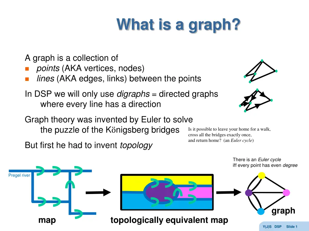
What is a graph? A graph is a collection of points (AKA vertices, nodes) lines (AKA edges, links) between the points In DSP we will only use digraphs = directed graphs where every line has a direction Graph theory was invented by Euler to solve the puzzle of the K onigsberg bridges Is it possible to leave your home for a walk, cross all the bridges exactly once, and return home? (an Euler cycle) But first he had to invent topology There is an Euler cycle iff every point has even degree Pregel river graph map topologically equivalent map Y(J)S DSP Slide 1

Topology? Topology is a generalization of geometry in geometry congruence allows translation and rotation Side Side Side Side Angle Side Angle Side Angle but not Angle Angle Angle in affine geometry we also allow scale changes (zoom) Side Side Side Side Angle Side Angle Side Angle Angle Angle Angle in projective geometry we allow any transformation from lines to lines (maintains collinearity) here all triangles are equivalent, but squares are different in topology we allow any transformation that doesn t tear or glue together space (think of drawing on a rubber sheet) Y(J)S DSP Slide 2

Some more topology Topology s equivalence relationship is called homeomorphism A homeomorphism is a continuous function from space to space with a continuous inverse function In topology distance, angle, and linearity are meaningless triangle = square = polygon = circle all curves that don t cross themselves are equivalent a figure 8 is not the same as a circle (would require a tear) (the number of holes is preserved) in 3D topology a sphere is equivalent to a cube but not to a donut What Euler realized is that the existence of a Euler cycle is independent of the bridge location and orientation The bridge puzzle is truly a topological problem Y(J)S DSP Slide 3

Continuous transformations Continuously morph a square into a circle (and back again) Continuously triangle into a square (and back again) Y(J)S DSP Slide 4

Topology and graph theory In graph theory all we care about is connectivity which point is connected to which point We don t care about the length or angle of the line or even if it is a line The meaning of a graph is purely topological So all the following digraphs are equivalent: y x x y x y y x y x But not or y x x w y Y(J)S DSP Slide 5

Graph theory in CS In the early days of computer science programs were represented by block diagrams which are a kind of graph processing This representation has been mostly abandoned for several reasons: block diagrams are actually a programming language so using them in addition to code means maintaining 2 code different sets block diagrams are tightly coupled to imperative program with goto statements which has been disparaged block diagrams are purely documentation and add nothing positive to the programming process block diagrams only describe algorithms Wirth s Law programs = algorithms + data structures false if true Goto A But in DSP we still use signal flow graphs! Y(J)S DSP Slide 6

Signal flow graphs Shannon introduced signal flow graphs in which the points represent signals the lines (and things on lines) represent signal processing functions These graphs capture both algorithms and data structures In addition to their purely documentary function signal flow graphs are useful because of graphical mechanisms for simplifying graphs lowering computational power or memory requirements Y(J)S DSP Slide 7

The simplest graph The simplest signal flow graph has 1 point and represents a signal x When we write a letter next to a point (below, left, right, above) it represents the name of the signal (here: x !) When interpreting signal flow graphs it is often useful to ask what is the value of the signals at time n ? So we sometime draw xn But don t be confused! The point represents the signal xn n= - + not a particular value Y(J)S DSP Slide 8

The next simplest graph The simplest nontrivial signal flow graph has 2 points and one line and it represents signal identity (y = x, i.e., n= - + yn = xn) identity = assignment x y y = x Of course, due to the topological nature of graphs we could have drawn this graph in many other ways y x x y y x And in this case only we can also reverse the line direction y x x y Note that we will often neglect to draw the point when it is obvious (i.e., at the end of a line) (we will later only draw points in specific places ) Y(J)S DSP Slide 9

What does this mean? y x y z x We can figure this out by naming the unlabeled point w and breaking the graph down into three parts x w w z So w = x and y = w = x and also z = w = x WARNING! Do not think of this as electrical currents in which case y=x/2 and z=x/2 ! y y = x and z = x x splitter = tee connector This graph is called the splitter z Note that the splitter always has 1 signal going in and 2 signals coming out Y(J)S DSP Slide 10

Gain The simplest signal processing is the gain y = g x ( n= - + yn = g xn) We draw this by putting the letter g next to the arrow x y gain g y = g x Note that (for g 1) this is very different from g x y y x x = g y but the same as etc. g g g g x x y y y x Be careful! A letter near a point tells you the signal s name but a letter near an arrow represents a gain Y(J)S DSP Slide 11

Delay We have seen that the unit delay is very important in DSP and so it deserves its own graphical symbol y x z-1 y = z 1 x( n= - + yn = xn-1 ) unit delay and as usual we can draw this in various orientations, such as x z-1 y x z-1 y g g y is the same as ? x y z-1 x z-1 Y(J)S DSP Slide 12

Drawing points We will always explicitly draw the point after a delay element z-1 Since this point represents a signal value that must be remembered that is, a memory location For this reason we frequently use the term memory point Marking memory points help us count up how much memory is required For example, we see that y = z 3 x requires 3 memory points x z-1 z-1 z-1 y Note: We will sometimes temporarily draw and label points just in order to understand the graph Y(J)S DSP Slide 13

Adder Signal addition is very important as well! We define the two-signal adder which of course means n= - + zn = xn + yn Note that the adder always has 2 signals going in and 1 signal coming out x z adder z = x + y y y As usual, we could draw the adder in many ways! y y z x z z x x Y(J)S DSP Slide 14

Subtractor For convenience we also define the 2-signal subtractor x z - z = x - y y Note the position of the minus sign It can be at either (or both) of the adder s inputs! Although we could have used instead x z -1 y Y(J)S DSP Slide 15

The finite difference We can now use what we have learned so far to draw a useful graph the finite difference y = x ( i.e., yn = xn - xn-1 ) yn n = xn n - xn n- -1 1 To see that this is correct label needed points (not just the memory points) with their value at time n xn n yn n splitter xn n- -1 1 xn n Y(J)S DSP Slide 16

The butterfly Remember the DFT for N=2 ? X0 = x0 + x1 X1 = x0 x1 We can draw this as a DSP graph (it is not really a signal flow graph!) Rotating this 90 degrees and using a lot of imagination one can understand why this is called a butterfly Y(J)S DSP Slide 17

The basic MA filter Let s draw something even more interesting yn n = a0 0 xn n + a1 1 xn n- -1 1 To see that this is indeed the MA filter label all these points yn n xn n a0 xn n a1 xn n- -1 1 xn n xn n- -1 1 Y(J)S DSP Slide 18

Basic MA blocks Here are 4 interesting ways to draw this same simple MA filter What transformations brings us from one to the other? topological topological commute yn n = a0 0 xn n + a1 1 xn n- -1 1 Y(J)S DSP Slide 19

Why do we need 4 blocks? Products next to adder can make memoryless chip Products all parallel easy to iterate (we ll see later) Products all parallel easy to iterate (we ll see later) y line is different height from x line Delay element adjacent to adder Y(J)S DSP Slide 20

Commutativity Note that it is obvious that the gain g and the delay z 1 commute but this is true more generally for any two filters While somewhat complicated to prove in the time domain it is simple to see in the frequency (or z) domain Since filters obey Y( ) = H( ) X( ) two filters f and g in series obey Y( ) = G( ) F( ) X( ) G( ) F( ) X( ) F( ) X( ) g f Y( ) X( ) while in the opposite order Y( ) = F( ) G( ) X( ) F( ) G( ) X( ) G( ) X( ) f g Y( ) X( ) which is the same thing since functions commute! Show 2 systems that do not commute Y(J)S DSP Slide 21

General MA Now we consider the general MA filter with L coefficients y a x L = = l n l n l 0 We would like to draw but we only defined 2-input adders ! Y(J)S DSP Slide 22

Tapped delay line Before correcting this, note that top of this diagram has an interesting analog interpretations Engineers think of this as a tapped delay line similar to a length of cable with finite transmission velocity But since information travels in (copper or optical) cables at 2/3 the speed of light (200 meters per sec) you need a long cable for significant delay ! tapped delay line Y(J)S DSP Slide 23

A data structure! We will think of this differently (and find a data structure in addition to the algorithm) Considering the memory points from some time we find a data structure (assume L=8) with the following time varying contents x y z-1 z-1 z-1 z-1 z-1 z-1 z-1 x6 x2 x7 x5 x6 x3 x1 x2 x8 x4 x5 x7 x3 x8 x4 x9 x8 x4 x9 x7 x8 x5 x3 x4 x10 x6 x7 x9 x5 x10 x6 x11 We see that values that enter first from the left exit (are discarded) first to the right so this is a FIFO buffer Y(J)S DSP Slide 24

How do we fix the adders So, were we to use an N-input adder we would have a FIFO, multiplications, and an adder FIFO Let s perform the additions one at a time! Y(J)S DSP Slide 25

General MA 1st way = l 0 a x L = y n l n l MACs We still have the tapped delay line = FIFO as a data structure but now we perform Multiplication + Accumulations (MACs) We have previously mentioned how important MACs are in DSP Another way of looking at this is iteration on one of our basic MA blocks Which one ? Y(J)S DSP Slide 26

Iteration 1st way = l 0 a x L = y n l n l MACs We iterate on basic block D So this graph tells us 1. Data structure = FIFO 2. Algorithm = iteration over MA block D Y(J)S DSP Slide 27

The signals point of view We saw how to look at this from the processing point of view Sometimes it is useful to look at graphs from the signal s point of view! the signal enters the filter and is split into 2 replicas : A and B gain is applied to replica A, replica B is delayed replica B is split in two : C and D gain is applied to replica C, which then is added to replica A etc. Y(J)S DSP Slide 28

General MA 2nd way This isn t the only way to compute a general MA Here we see an alternative It still uses a FIFO data structure (which is now vertical but who cares?) Which basic MA block is used here? So this graph tells us 1. Data structure = FIFO 2. Algorithm = iteration over MA block A FIFO MACs Y(J)S DSP Slide 29

Two ways to MA Is there any difference between these two ways? the 1st way MACs from the new x backward a0 xn + a1 xn-1+ + aL xn-L the 2nd way MACs from the earliest x forward aL xn-L+ + a1 xn-1 + a0 xn Theoretically there is no difference (addition is commutative) but in practice there may be Given a list of numbers sorted from smallest to largest which way is most accurate to sum? Y(J)S DSP Slide 30

Basic AR block = + y x by What is the graph for the basic AR filter ? Here is one way: 1 n n n Note that for the first time we see a loop in the graph in none of the MA filters was there a loop! Whenever there is a loop, there is recursion (AR) Put another way loops correspond to poles Y(J)S DSP Slide 31

How does it work? As usual let s label points to see why this works yn n xn n xn n + b yn n- -1 1 = + y x by 1 n n n yn n yn n- -1 1 b yn n- -1 1 We don t worry about signals from the past influencing the output now but non-causal loops can be paradoxical (like time travel) This is just one way the draw the simple AR there are 4 basic blocks here too Can you find them? Y(J)S DSP Slide 32

A loop with no delay It can be useful (but dangerous) to make a loop with no delay Consider an amplifier which has some of the output fed back into the input g x y g x y b Then instead of y = g x we have y = g(x+by) or y bgy= gx and hence y = g 1 bgx So the feedback increases the amplifier s gain when b < 1/g but explodes as b 1/g We see here the connection between loops and poles! The same thing happens with delay but only for certain frequencies! Y(J)S DSP Slide 33

General AR filters Here are two ways to implement the general AR filter b y M = + = m y x n n m n m 1 Explain why these indeed implement the AR Is there any difference between these two ways? Y(J)S DSP Slide 34

ARMA filters stage 1 a x b y L M = + l = l = m y What do we do about ARMA filters? The straightforward implementation would be perform the MA portion using one of our MA implementations perform the AR portion using one of our AR implementations add the two together n l n m n m 0 1 a x b y L M = + l = l = m y n l n m n m MA AR 0 MA 1 + AR Y(J)S DSP Slide 35

How much memory? u a x b y L M = + l = l = m y n l n m n m 0 1 By observing the graph we see that L+M memory points are used Without limiting generality we can say 2L memory points and assume L=M Why? Take max(L,M) and pad the other with zeros We will now use graph theory to reduce the number of needed memory points Y(J)S DSP Slide 36

ARMA filters stage 2 w a x b y L M = + l = l = m y n l n m n m 0 1 The graph has two filters in series 1 MA and 1 AR Since any 2 filters commute we can exchange their order We obtain this new graph Note that the signal w between the 2 filters is different from the signal u ! Y(J)S DSP Slide 37

ARMA filters stage 3 wn a x b y L M = + l = l = m y n l n m n m wn-1 0 1 We see that there are points representing the same signal ! wn-2 All of these are So we can combine the memory locations and remove un-needed delays This is a new graph transformation Y(J)S DSP Slide 38

ARMA filters stage 3 a x b y L M = + l = l = m y n l n m n m 0 1 We now require only L memory points instead of 2L memory points A reduction to 50% ! Y(J)S DSP Slide 39

The transposition theorem Another transformation that creates a new graph that is equivalent in functionality to the original one is given by the Transposition theorem This transformation is more complex since multiple operations are carried out at the same time exchange input(s) and output(s) reverse direction of all arrows replace adders with splitters (since now 1 in - 2 out) replace splitters with adders (since now 2 in - 1 out) Y(J)S DSP Slide 40

2 simple cases a0 a0 x y y x Simple MA z-1 z-1 a1 a1 a0 x y y x Simple AR z-1 z-1 b1 b1 Y(J)S DSP Slide 41

Summary the 4 transformations We have learned 4 basic transformations that create equivalent signal flow graphs 1. transformations that do not change topology 2. changing order of filters 3. identification of identical signal points and removal of redundant branches 4. the transposition theorem These transformations can be carried out mechanically and are used to reduce the amount of memory needed (we saw such a case!) reduce the amount of computation needed (we ll see next time) This is why graphs are still used in DSP ! Y(J)S DSP Slide 42