Traffic Fatality Rate and Crime Rate Analysis in Nebraska and Colorado
Explore the impact of policy implementations on traffic fatality rates and crime rates in Nebraska and Colorado using a Difference-in-Difference model. Estimating equations and results are presented for both traffic fatality rates and crime rates, shedding light on the effects of the interventions over time.

Download Presentation

Please find below an Image/Link to download the presentation.
The content on the website is provided AS IS for your information and personal use only. It may not be sold, licensed, or shared on other websites without obtaining consent from the author. If you encounter any issues during the download, it is possible that the publisher has removed the file from their server.
You are allowed to download the files provided on this website for personal or commercial use, subject to the condition that they are used lawfully. All files are the property of their respective owners.
The content on the website is provided AS IS for your information and personal use only. It may not be sold, licensed, or shared on other websites without obtaining consent from the author.
E N D
Presentation Transcript
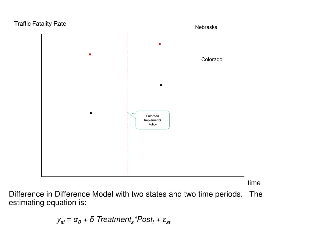
Traffic Fatality Rate Nebraska Colorado Colorado Implements Policy time Difference in Difference Model with two states and two time periods. The estimating equation is: yst= 0+ Treatments*Postt+ st
Crime Rate Nebraska Average yst is 0 Average ystis 0 + (Note here that is negative) Colorado Colorado Implements Policy time Suppose the estimating equation is: yst= 0 + Treatedst + st
Crime Rate Nebraska Average yst is 0 Average ystis 0 + (Note here that is negative) Colorado Colorado Implements Policy time Suppose the estimating equation is: yst= 0 + Treatedst + st
Traffic Fatality Rate Nebraska Colorado Colorado Implements Policy time Difference in Difference Model with two states and two time periods. The estimating equation is: yst= 0+ 1Treatments + Treatments*Postt + st
Traffic Fatality Rate Nebraska 0 Colorado 0 + 1 + 0+ 1 Colorado Implements Policy time Difference in Difference Model with two states and two time periods. The estimating equation is: yst= 0+ 1Treatments + Treatments*Postt + st
Traffic Fatality Rate Nebraska 0 Colorado 0 + 1 + 0+ 1 Colorado Implements Policy time Difference in Difference Model with two states and two time periods. The estimating equation is: yst= 0+ 1Treatments + Treatments*Postt + st
Traffic Fatality Rate Nebraska Colorado Colorado Implements Policy time Difference in Difference Model with two states and two time periods. The estimating equation is: yst= 0+ 1Treatments+ 2Postt + + Treatments*Postt + st
Traffic Fatality Rate Nebraska Colorado Colorado Implements Policy time Difference in Difference Model with two states and two time periods. The estimating equation is: yst= 0+ 1Treatments + + 2Postt + Treatments*Postt + st
Traffic Fatality Rate Nebraska 2 Colorado 2+ 0 Colorado Implements Policy 0+ 1 time Difference in Difference Model with two states and two time periods. The estimating equation is: yst= 0 + 1Treatments+ 2Postt + + Treatments*Postt + st
Traffic Fatality Rate Nebraska 2 Colorado 2 0 Colorado Implements Policy 0+ 1 time Difference in Difference Model with two states and two time periods. The estimating equation is: yst= 0 + 1Treatments+ 2Postt + + Treatments*Postt + st
Traffic Fatality Rate Nebraska 2 Colorado . 2 Colorado Implements Policy time Difference in Difference Model with two states and two time periods. The estimating equation is: yst= 0+ 1Treatments+ 2Postt + + Treatments*Postt + st
Traffic Fatality Rate Nebraska 2 Colorado . 2 Colorado Implements Policy time This estimating equation is exactly the same as: yist= 0 + 1dCOs + 2d2t + + Policyst + ist dCO is dummy for CO; d2 is dummy for year 2; Policy is dummy =1 in CO after policy is passed
Traffic Fatality Rate Nebraska Colorado . Colorado Implements Policy time ???? ??= 2d2t + + Policyst +???? ??
Traffic Fatality Rate Colorado . Nebraska 2 time The estimate of is exactly the same as obtained by subtracting the mean for each state: ???? ??= 2d2t + + Policyst +???? ??
Traffic Fatality Rate Colorado . Nebraska time And is exactly the same after subtracting the mean for each time period: ???? ?? ??= Policyst +???? ?? ??
When we have lots of states and years, an author typically writes yst = 0 + Policyst + vs + zt + st And then the author might say that the equation is estimated including state and year fixed effects Start with state fixed effects, common time trend
Traffic Fatality Rate Nebraska Colorado . Colorado Implements Policy 0 0 + 1 time If we re using state-level data, then each state contributes one observation per year. The estimating equation with a common time trend is yist= 0+ 1dCOs + 2t + Policyst + ist
Traffic Fatality Rate Colorado Nebraska . Colorado Implements Policy time Remove state specific means will still be the vertical change ???? ??= 2t + Policyst + ???? ??
Traffic Fatality Rate Nebraska Colorado New Mexico . Colorado Implements Policy . New Mexico Implements Policy time With multiple states will be the average vertical change across the states yst= 0 + 2 t + Policyst + vs + st
Traffic Fatality Rate Nebraska . Colorado New Mexico .. Colorado Implements Policy . New Mexico Implements Policy time If we re using repeated cross-sectional data at the individual level, then each state contributes multiple observations per year. The estimating equation is: yist= 0 + Policyst+ 2 t + vs + ist
Pooled model: MRit = 0 +1unemit +eit murder rate 11.1 17.2 20.3 id 19 19 19 state year LA LA LA unem 12 6.2 7.4 87 90 93 5 5 5 CA CA CA 87 90 93 10.6 11.9 13.1 5.8 5.6 9.2
FD model: MRit = 1unemit + eit murder rate 11.1 17.2 20.3 id 19 19 19 state year LA LA LA MR -- 6.1 3.1 unem UN 12 6.2 7.4 87 90 93 -- -5.8 1.2 5 5 5 CA CA CA 87 90 93 10.6 11.9 13.1 -- 5.8 5.6 9.2 -- 1.3 1.2 -.02 3.6
FE model: MRit -???= 1unemit????i + eit UN- mean murder rate 11.1 17.2 20.3 MR- mean unemmean -5.1 12 1 6.2 4.1 7.4 id state year 19 LA 19 LA 19 LA Mean 16.2 16.2 16.2 87 90 93 8.5 8.5 8.5 3.5 -2.3 -1.1 5 5 5 CA CA CA 87 90 93 10.6 11.9 13.1 11.9 11.9 11.9 -1.3 0 1.2 5.8 5.6 9.2 6.9 6.9 6.9 -1.1 -1.3 2.3
The estimated coefficient on unemployment from these two models will be the same if there are only 2 years. Otherwise, they are both consistent estimators of 1 but their exact values will differ
FE model: MRit = 0+1unemit + 1Statei +eit murder rate unem 11.1 17.2 20.3 id state year 19 LA 19 LA 19 LA State 1 1 1 87 90 93 12 6.2 7.4 5 5 5 CA CA CA 87 90 93 10.6 11.9 13.1 5.8 5.6 9.2 0 0 0
FE model: MRit = 0+1unemit + 1Statei +eit murder rate unem 11.1 17.2 20.3 id state year 19 LA 19 LA 19 LA State 1 1 1 The constant term in this model and the previous version of the FE model will be different (how?) 87 90 93 12 6.2 7.4 The estimated coefficient on unemployment WILL BE EXACTLY THE SAME 5 5 5 CA CA CA 87 90 93 10.6 11.9 13.1 5.8 5.6 9.2 0 0 0
Now look at time shocks. What if all states experience a common shock in a given year? What if the means varies by time as well as by state?
Crime Rate . Jefferson legalizes by-the-drink sales z8 Jefferson z3 z8 Barber Barber legalizes by-the-drink sales z3 time Negative shock to crime Positive shock to crime Common time fixed effects-- will still be the average vertical change from before and after the policy Violent Crimect = 0 + Wet Lawct + X ct 2 + vc + zt+ ct
Crime Rate . Jefferson legalizes by-the-drink sales z8 Jefferson z3 z8 Barber Barber legalizes by-the-drink sales z3 time Negative shock to crime Positive shock to crime Common time fixed effects-- will still be the average vertical change from before and after the policy Violent Crimect = 0 + Wet Lawct + X ct 2 + vc + zt+ ct
Crime Rate . Jefferson legalizes by-the-drink sales Jefferson Barber Barber legalizes by-the-drink sales time Negative shock to crime Positive shock to crime But note if you look at it, Barber is increasing faster than Jefferson: Violent Crimect = 0 + 1Wet Lawct + X ct 2 + vc + zt+ ct
Crime Rate . Jefferson legalizes by-the-drink sales Jefferson Franklin Barber Barber legalizes by-the-drink sales Franklin legalizes by-the- drink sales time Negative shock to crime Positive shock to crime Adding state specific time trends Violent Crimect = 0 + Wet Lawct + X ct 2 + vc + zt+ c t + ct
Meyer et al. Workers compensation State run insurance program Compensate workers for medical expenses and lost work due to on the job accident Premiums Paid by firms Function of previous claims and wages paid Benefits -- % of income w/ cap 35
Typical benefits schedule Min( pY,C) P=percent replacement Y = earnings C = cap e.g., 65% of earnings up to $400/month 36
Concern: Moral hazard. Benefits will discourage return to work Empirical question: duration/benefits gradient Previous estimates Regress duration (y) on replaced wages (x) Problem: given progressive nature of benefits, replaced wages reveal a lot about the workers Replacement rates higher in higher wage states 37
Yi = Xi + Ri + i Y (duration) R (replacement rate) Expect > 0 Expect Cov(Ri, i) Higher wage workers have lower R and higher duration (understate) Higher wage states have longer duration and longer R (overstate) 38
Solution Quasi experiment in KY and MI Increased the earnings cap Increased benefit for high-wage workers (Treatment) Did nothing to those already below original cap (comparison) Compare change in duration of spell before and after change for these two groups 39
Model Yit = duration of spell on WC Ait = period after benefits hike Hit = high earnings group (Income>E3) Yit = 0 + 1Hit + 2Ait + 3AitHit + 4Xit + it Diff-in-diff estimate is 3 42
Questions to ask? What parameter is identified by the quasi-experiment? Is this an economically meaningful parameter? What assumptions must be true in order for the model to provide and unbiased estimate of 3? Do the authors provide any evidence supporting these assumptions? 44
Almond et al. Neonatal mortality, dies in first 28 days Infant mortality, died in first year Babies born w/ low birth weight(< 2500 grams) are more prone to Die early in life Have health problems later in life Educational difficulties generated from cross-sectional regressions 6% of babies in US are low weight Highest rate in the developed world 45
Let Yit be outcome for baby t from mother I e.g., mortality Yit = + bwit + Xi + i + it bw is birth weight (grams) Xi observed characteristics of moms i unobserved characteristics of moms 46
Cross sectional model is of the form Yit = + bwit + Xi + uit where uit = i + it Many observed factors that might explain health (Y) of an infant Prenatal care, substance abuse, smoking, weight gain (of lack of it) Some unobserved as well Quality of diet, exercise, generic predisposition i not included in model Cov(bwit,uit) < 0 47
Solution: Twins Possess same mother, same environmental characterisitics Yi1 = + bwi1 + Xi + i + i1 Yi2 = + bwi2 + Xi + i + i2 Y = Yi2-Yi1 = (bwi2-bwi1) + ( i2- i1) 48
Questions to consider? What are the conditions under which this will generate unbiased estimate of ? What impact (treatment effect) does the model identify? 49