Transfer Functions and Control Systems in Engineering

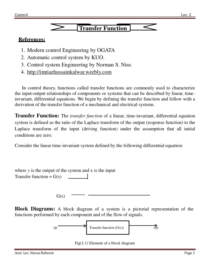
Control Lec. 2 Transfer Function References: 1. Modern control Engineering by OGATA 2. Automatic control system by KUO. 3. Control system Engineering by Norman S. Nise. 4. http://imtiazhussainkalwar.weebly.com In control theory, functions called transfer functions are commonly used to characterize the input-output relationships of components or systems that can be described by linear, time- invariant, differential equations. We begin by defining the transfer function and follow with a derivation of the transfer function of a mechanical and electrical systems. Transfer Function: The transfer function of a linear, time-invariant, differential equation system is defined as the ratio of the Laplace transform of the output (response function) to the Laplace transform of the input (driving function) under the assumption that all initial conditions are zero. Consider the linear time-invariant system defined by the following differential equation: where y is the output of the system and x is the input Transfer function = G(s) | G(s) Block Diagrams: A block diagram of a system is a pictorial representation of the functions performed by each component and of the flow of signals. i/p Transfer function (G(s)) o/p Fig(2.1) Element of a block diagram Asst. Lec. Haraa Raheem Page 1

Control Lec. 2 Summing Point: Acircle with a cross is the symbol that indicates a summing operation. a a-b b Fig (2.2) Summing point Branch Point: A branch point is a point from which the signal from a block goes concurrently to other blocks or summing points. Block Diagram of a Closed-Loop System: Figure (2.3) shows an example of a block diagram of a closed-loop system. The output C(s) is fed back to the summing point, where it is compared with the reference input R(s). The closed-loop nature of the system is clearly indicated by the figure. The output of the block, C(s) in this case, is obtained by multiplying the transfer function G(s) by the input to the block, E(s). Any linear control system may be represented by a block diagram consisting of blocks, summing points, and branch points. Fig (2.3) Block diagramof a closed-loop system When the output is fed back to the summing point for comparison with the input, it is necessary to convert the form of the output signal to that of the input signal. This conversion is accomplished by the feedback element whose transfer function is H(s), as shown in Figure (2.4). Fig (2.4) Closed-loop system Asst. Lec. Haraa Raheem Page 2

Control Lec. 2 Referring to Figure (2.4), the ratio of the feedback signal B(s) to the actuating error signal E( s ) is called the open-loop transfer function. That is, Open-loop transfer function The ratio of the output C(s) to the actuating error signal E(s) is called the feedforward transfer function, so that Feedforward transfer function If the feedback transfer function H(s) is unity, then the open-loop transfer function and the feedforward transfer function are the same. In Figure (2.4), the output C(s) and input R(s) are related as follows: since [ ] 2.2 Mathematical Models of System Mathematical model: The mathematical description of the dynamic characteristics of a system is called mathematical model or mathematical model is the representation of the dynamic behavior of a physical system by a set of equations. The first step in the analysis of a dynamic system is to drive its model. Asst. Lec. Haraa Raheem Page 3

Control Lec. 2 2.2.1 Electric circuits and components The basic passive elements of electrical systems are resistance, inductance and capacitance. 1-- Resistance The time domain expression relating voltage and current for the resistor is given by Ohm s law i-e The Laplace transform of the above equation is VR(s) = IR(s)R 2- The time domain expression relating voltage and current for the Capacitor is given as: 1 ic (t)dt vc (t) = C Asst. Lec. Haraa Raheem Page 4

Control Lec. 2 The Laplace transform of the above equation (assuming there is no charge stored in the capacitor) is 1 V (s ) = I (s ) c c C s 3- The time domain expression relating voltage and current for the inductor is given as: Ld iL(t (t ) = ) vL d t The Laplace transform of the above equation (assuming there is no energy stored in inductor) is VL(s) = LsIL(s) Table (2.1) Asst. Lec. Haraa Raheem Page 5

Control Lec. 2 Basic laws governing electrical circuits are Kirchhoff's current law and voltage law, which state: 1.Sum of currents entering a node is equal to the sum of currents leaving the same node. 2. The algebraic sum of the voltages around any loop in an electrical circuit is zero. A mathematical model of an electrical circuit can be obtained by applying one or both of Kirchhoff's laws to it. For the series RLC circuit shown below: i(t) V(t) Applying Kirchhoff's voltage law to the system, we obtain the following equations: (2.9) A transfer function model of the circuit can also be obtained as follows: Taking the Laplace transforms of Equation (2.9), assuming zero initial conditions, we obtain [ ] is assumed to be the input and system is found to be If , the output, then the transfer function of this Asst. Lec. Haraa Raheem Page 6

Control Lec. 2 For the parallel RLC circuit shown below: Applying Kirchhoff's current law to the system, we obtain the following equations: [ ] If system is found to be is assumed to be the input and , the output, then the transfer function of this Asst. Lec. Haraa Raheem Page 7

Control Lec. 2 Ex1: Consider the system shown in Figure.Assume that ei is the input and eo, is the output. The equations for this system are: Taking the Laplace transforms of Equations, using zero initial conditions, we obtain (1) (2) Eliminating I1(s) from Equations (1) and (2) and writing Ei(s) in terms of I2(s), we find the transfer function between Eo(s) and Ei(s) to be H.W/ Given the network of Figure below , find the transfer function, Asst. Lec. Haraa Raheem Page 8

Control Lec. 2 2.2.2.1 Mechanical translation system In this section we shall discuss mathematical modeling of mechanical systems. The fundamental law governing mechanical systems is Newton's second law. It can be applied to any mechanical system. The elements of Mechanical system are mass, spring and dashpot. 1. Mass (M) F Mass x(t) a force applied to the mass produce an acceleration of the mass. Fmis equal to the product of mass and acceleration. where a= acceleration v= velocity d i s p l acement at any time (t) D-operator = Fd 2. Dashpot Adamping element (sometimes called a dashpot) is assumed to produce a velocity proportional to the force applied to it. x(t) where B is damping factor Asst. Lec. Haraa Raheem Page 9

Control Lec. 2 3. Spring: A translational spring is a mechanical element that can be deformed by an external force such that the deformation is directly proportional to the force applied to it. Circuit Symbols Translational Spring The elastance, or stiffness k provides a restoring force as represented by a spring where k is elastance of spring TABLE 2.2 Force-velocity, force-displacement, and impedance translational relationships for springs, viscous dampers, and mass Asst. Lec. Haraa Raheem Page 10

Control Lec. 2 Mechanical systems parallel electrical networks to such an extent that there are analogies between electrical and mechanical components and variables. Mechanical systems, like electrical networks, have three passive, linear components. Two of them, the spring and the mass, are energy-storage elements; one of them, the viscous damper, dissipates energy. The two energy-storage elements are analogous to the two electrical energy-storage elements, the inductor and capacitor. The energy dissipater is analogous to electrical resistance. Ex 1: Find the transfer function X2(s)/F(s) of the following system x2 x1 k B M F The Mechanical Network of this system is k x1 x2 At node x1 F = k(x1 x2) (1) F B M At node x2 0 = k(x2 x1) + M x 2 + Bx 2 (2) Taking Laplace transfer for equations 1& 2 (5) [ ] From equation (3) (6) Asst. Lec. Haraa Raheem Page 11

Control Lec. 2 Substitute equ. (6) in (5) [ ] ] [ [ ] [ ] [ ] [ ] Ex 2: Write the differential equation for the system x1 x2 B3 B4 k M1 M2 f ( t ) B1 B2 The Mechanical Network of this system is x1 B3 x2 B1 f (t) M2 M1 k B2 B4 Asst. Lec. Haraa Raheem Page 12

Control Lec. 2 At node x1 At node x2 H.W 1: Find the transfer function X1(s)/F(s) of the following system H.W 2: Find the transfer function X1(s)/F(s) of the following system Asst. Lec. Haraa Raheem Page 13