Transmission Lines in Frequency Domain for Communication Systems
Explore the importance of the frequency domain in communication systems, how solutions are derived using Fourier transform methods, and the significance of phasor domain analysis in solving for time-varying signals on transmission lines. Learn about Telegrapher's equations and the transfer function in the frequency domain.

Download Presentation

Please find below an Image/Link to download the presentation.
The content on the website is provided AS IS for your information and personal use only. It may not be sold, licensed, or shared on other websites without obtaining consent from the author. If you encounter any issues during the download, it is possible that the publisher has removed the file from their server.
You are allowed to download the files provided on this website for personal or commercial use, subject to the condition that they are used lawfully. All files are the property of their respective owners.
The content on the website is provided AS IS for your information and personal use only. It may not be sold, licensed, or shared on other websites without obtaining consent from the author.
E N D
Presentation Transcript
ECE 3317 Applied Electromagnetic Waves Prof. David R. Jackson Fall 2024 Notes 9 Transmission Lines (Frequency Domain) 1
Frequency Domain Why is the frequency domain important? Most communication systems use a sinusoidal signal (which may be modulated). (Some systems, like Ethernet, communicate in baseband , meaning that there is no carrier.) Examples: 100BASET, 10GBASET 2
Frequency Domain (cont.) Why is the frequency domain important? A solution in the frequency-domain allows to solve for an arbitrary time-varying signal on a lossy line (by using the Fourier transform method). Fourier-transform pair For a physically-realizable (real-valued) signal, we can also write j t ( ) = ( ) v t e v dt 1 1 = j t ( ) ( ) v t Re v e d j t = ( ) ( ) v t v e d 2 0 ( ) ( ) ( ) = * since v v Jean-Baptiste-Joseph Fourier 3
Frequency Domain (cont.) 1 j t = ( ) Re ( ) v t v d e A collection of phasor-domain signals! 0 Phasor ( ) v t 1.0 A pulse is resolved into a collection (spectrum) of infinite sinusoidal waves with different frequencies, amplitudes, and phases. t W V t Time 4
Frequency Domain (cont.) Example: Rectangular pulse = j t ( ) ( ) v t e v dt ( ) v t 1.0 t W ( ) ( ) = sinc /2 v W W ( ) x x sin ( ) x sinc 5
Frequency Domain (cont.) System ( ) H ( ) ( ) Phasor domain: V V in out In the frequency domain, the system has a transfer function H( ): ( ) out V ( ) ( ) = H V in System ( ) t ( ) ( ) t H v Time domain: v in out The time-domain response of the system to an input signal is: 1 ( ) = j t ( ) ( ) t Re v H v e d out in 0 6
Frequency Domain (cont.) Summary Phasordomain: ( ) ( ) V V ( ) out H System in ( ) t ( ) ( ) t H v v in out 1 ( ) = j t ( ) ( ) t Re v H v e d out in 0 If we can solve the system in the phasor domain (i.e., get the transfer function H( )), we can get the output for any time-varying input signal. This is one reason why the phasor domain is so important! This applies for transmission lines also! 7
Telegraphers Equations 2 2 v v t v ( ) + = ( ) 0 RG v RC LG LC 2 2 z t L z R z ( ) + , i z t ( ) , v z t G z C z - z z 8
Frequency Domain j To convert to the phasor domain, we use: t 2 2 v v t v ( ) + = ( ) 0 RG v RC LG LC 2 2 z t 2 V z ( ) ( ) 2 + = ( ) 0 RG V j RC LG V j LCV 2 or 2 d V dz ( ) ( ) = + + 2 ( ) RG V j RC LG V LC V 2 9
Frequency Domain (cont.) 2 d V dz ( ) ( ) = + + 2 ( ) RG j RC LG LC V 2 Note that + + = + j L G + j C 2 ( ) ( )( ) RG j RC LG LC R = = + + = = Z Y R G j L j C series impedance / length parallel admittance / length 2 d V dz = ( ) ZY V We can therefore write: 2 10
Telegraphers Equations 2 d V dz = ( ) ZY V 2 = + j L Z R = + j C Y G L z R z + ( ) V z G z C z - z z 11
Frequency Domain (cont.) 2 d V dz = ( ) ZY V 2 Define = + j L G + j C 2 ( )( ) ZY R Then 2 d V dz = 2 ( ) V 2 Solution: + = + z z ( ) V z Ae Be Note: We have an exact solution, even for a lossy line, in the phasor domain! 12
Propagation Constant Convention: We choose the (complex) square root to be the principal branch: + j L G + j C ( )( ) R (lossy case) is called the propagation constant, with units of [1/m] Review of principal branch of square root: Note: = /2 /2 /2 j c c e ( ) /2 j = c c e c Re 0 13
Propagation Constant (cont.) = + j L G + j C ( )( ) R = + j Denote: = propagation constant [1/m] = attenuation constant [nepers/m] = phase constant [radians/m] Choosing the principal branch means that 0 Re 0 14
Propagation Constant (cont.) For a lossless line, we consider this as the limit of a lossy line, in the limit as the loss tends to zero: ( ) = + j L G + j C = ( )( ) 1 R LC = j LC (lossless case) Hence Hence, we have that = = 0 LC Note: = 0 for a lossless line. 15
Propagation Constant (cont.) Physical interpretation of waves: + = = z ( ) z ( ) z V V Ae Be (forward traveling wave) Note: The waves must decay in the direction of propagation. + z (backward traveling wave) = + j + j z = z ( ) z V Ae e Forward traveling wave: (decaying as it travels) + + j z = z ( ) z V Be e (decaying as it travels) Backward traveling wave: 16
Propagation Wavenumber Alternative notations: = + j (propagation constant) = zk j (propagation wavenumber) = Note: jk z + j z = = = jk z z z ( ) z V Ae Ae Ae e z 17
Forward Wave + j z = z ( ) z V Ae e Forward traveling wave: = j A A e Denote + j z = j z ( ) z V A e e e Then In the time domain we have: ( ) z e + + j t = ( , ) Re v z t V + = + z ( , ) z t cos( ) v A e t z Hence, we have 18
Forward Wave (cont.) + = + z ( , ) z t cos( ) v A e t z Snapshot of Waveform: t = 0 g z A e z The distance gis the distance it takes for the waveform to repeat itself in meters. g= guided wavelength 19
Wavelength The wave repeats (except for the amplitude decay) when: = 2 g 2 = Hence: g Note: This equation can be used to find g if we already know : 2 2 2 = = = ( ) ( ) g Im + j L G + j C Im ( )( ) R 20
Wavelength (cont.) Lossless case: 2 2 2 f 1 1 1 f c c = = = = = = = = = 0 d f g d 2 LC LC f LC f r r r r Summary for lossless case: = g d = 0 d = wavelength in dielectric d r r c f = 0 = wavelength in free-space (air) 0 c 8 2.99792458 10 m/s 21
Attenuation Constant The attenuation constant controls how fast the wave decays. + = + z ( , ) z t cos( ) v A e t z = z envelope A e t = 0 g z A e z ( ) ( ) = = + j L G + j C Re Re ( )( ) R 22
Phase Velocity The forward-traveling wave is moving in the positive z direction. Consider a sinusoidal wave moving on a transmission line (shown in the figure below for a lossless line ( = 0) for simplicity): + = + z ( , ) cos( ) v z t A e t z = = t t t t ( ) p v = velocity + 1 , v z t 2 m z + = 0 t z Crest of wave: 23
Phase Velocity (cont.) The phase velocity vphase is the velocity of a point on the wave, such as the crest. = = constant t z Set dz dt = 0 Take the derivative with respect to time: dz dt Hence = We thus have = phase v Note: This result holds for a general lossy line. ( ) = + j L G + j C Recall : Im ( )( ) R 24
Phase Velocity (cont.) Let s calculate the phase velocity for a lossless line: 1 LC Lossless line: = = = phase v = = 0 LC LC 1 c = = LC Also, we know that 2 d Recall: = phase v c Hence (lossless line) For a lossless line, any signal travels at the speed cd. (So this must be true for a sinusoidal signal!) d 1 1 1 c = = = Recall: c d 0 0 r r r r 25
Backward Traveling Wave Let s now consider the backward-traveling wave (shown in the figure below for a lossless line ( = 0) for simplicity): + + + j z j + + j z = = = B e z z z = ( ) z j V Be Be e B e e e B Denote + = + + z ( , ) cos( ) v z t B e t z ( ) = = t t t t p v = velocity , v z t 1 2 m z This wave has the same phase velocity, but it travels backwards. 26
Group Velocity The group velocity vgroup is the velocity of a pulse. gv z Note: We have (derivation omitted): For a lossy line, the pulse will be distorting as it propagates down the line. d d = group v Note: for a lossless line we have: = = = = 1/ 1/ group v phase v LC c d ( ) = = Lossless line: / 1/ LC d d LC 27
Attenuation in dB/m + j z = = = jk z z z ( ) z V Ae Ae Ae e z + ( ) (0) V V z = = z dB 20log 20log ( ) e Gain in dB: 10 10 + ln ln10 x x = log Use the following logarithm identity: 10 ( ) z ln e ( ) 20 ln10 z = = = dB 20 20 z Therefore, the gain is: ln10 ln10 20 ln10 = Attenuation [dB/m] Hence, we have: 28
Attenuation in dB/m (cont.) Final attenuation formulas: 20 ln10 = Attenuation [dB/m] ( ) Attenuation 8.686 [dB/m] 29
Example: Coaxial Cable 2 = F/m C 0 b a r Copper conductors (nonmagnetic: m= 0 ) ln b a = ln H/m L 0 = = 0.5 mm r a a 2 3.2 mm 2.2 = = b 2 b = S/m G d z b a = ln r TV coax = tan 0.001 = d 5.8 10 S/m 7 ma mb 1 1 ( ) = + /m R UHF 500 MHz f 2 2 a b ma ma mb mb Note: 2 2 The loss tangent of the dielectric is called tan d. = = ma mb ma ma mb mb (skin depth of the two conductors) 30
Example: Coaxial Cable (cont.) Dielectric conductivity is often specified in terms of the loss tangent: = tan d d d 0 r d = effective conductivity of the dielectric material* Note: The loss tangent of practical insulating materials (e.g., Teflon) is approximately constant over a wide range of frequencies. (For example, tan d 0.001for Teflon.) *The effective conductivity accounts for the actual conductivity as well as molecular friction and other effects. 31
Example: Coaxial Cable (cont.) Relation between G and C 2 = F/m C 0 b a r ln r a = G C d 2 b = S/m G d 0 r b a z ln G C = d 0 r Hence Recall G C = tan = tan d d d d 0 r This relationship holds for any type of transmission line. 32
Example: Coaxial Cable (cont.) Characteristic impedance (ignore R and G for this): L C b a = = ln 0 Z 0 2 r Z = 75 [ ] r a 0 b Skin depth of metal: z 2 = = ( ) 0.5 mm a = = m 0 m 3.2 mm 2.2 = = b = = 6 2.955 10 [m] r m = tan 0.001 = d 5.8 10 S/m 7 Effective conductivity of dielectric: ma mb ( ) ( ) UHF 500 MHz f = tan 0 d r d = 5 6.12 10 [S/m] d 33
Example: Coaxial Cable (cont.) = = 0.5 mm a 3.2 mm 2.2 = = b = r = tan 0.001 = d r a 5.8 10 S/m 7 ma mb b ( ) UHF 500 MHz f z = + j L G + j C ( )( ) R Results for (R,L,G,C): ) ( = + 0.022 15.543 1/m j H/m = = = = 2.147 /m R = = 0.022 nepers/m 15.544 rad/m 7 3.713 10 L 4 2.071 10 S/m G = Attenuation 0.191 dB/m 0.404 m 11 6.593 10 F/m C g = 34
Current Use the first Telegrapher equation: v z i t = Ri L j t V z = j LI RI Next, use + = + z z ( ) V z Ae Be V z ( ) z + = z z Ae Be so 35
Current (cont.) Hence, we have + = j LI z z Ae Be RI Solving for the phasor current I, we have + = z z I Ae Be + j L R ( )( j L ) + + j C R j L G R + + = z z Ae Be + + G R j C j L + = z z Ae Be 36
Characteristic Impedance Define the (complex) characteristic impedance Z0in the frequency domain for a lossy line: + + R G j L j C Z 0 Then we have: 1 Z + = z z ( ) I z Ae Be 0 Note: In the time domain, we only defined Z0 for a lossless line. In the frequency domain, we can define it for a lossy line. 37
Characteristic Impedance (cont.) ( ) I z Note the reference directions! + - ( ) ( ) z + V z V z + ( ) z V I = Z The characteristic impedance is the ratio of the voltage to the current, for a wave traveling in the positive z direction. ( ) z 0 + Practical note: Even though Z0 is always complex for a practical line (due to loss), we usually neglect this and take it to be real. + + R G j L j C L C = Z 0 38
Summary of Solution Characteristic Impedance Lossy Lossless: + + R G j L j C L C = Z = Z 0 0 Voltage and Current + = + z z ( ) V z Ae Be 1 Z + = z z ( ) I z Ae Be 0 39
Numerical Solution for Lossy Line System Phasordomain: ( ) t ( ) ( ) t H v ( ) ( ) v V V in ( ) out out H in 1 ( ) = j t ( ) ( ) t Re This must be evaluated numerically (e.g., using MATLAB). v H v e d out in 0 Lossy transmission line: + - ( ) ( ) z = + z z z = V z V 0 0 z ( )( ) ( ) R j L G j C + + z = = z H e e 0 0 40
Numerical Solution for Lossy Line (cont.) Example: Propagation on a lossy microstrip line (From ECE 5317) y x w t z + r ( ) z sv t Probe h Probe Coax SIDE VIEW TOP VIEW Input signal: = 2.33 = = = = s r = 0.5 10 10 t 0 tan h 0.001 1.0 ( ) 0.787 mm 31mils ( ) t gv 2.35 mm w ( ) 0.0175 mm t "half oz" copper cladding t = 3.0 10 S/m 7 0t m 41
Numerical Solution for Lossy Line (cont.) Example: Propagation on a microstrip line z = 20 cm z = 1 cm = 2.33 = = = = r tan h 0.001 z = 100 cm ( ) 0.787 mm 31mils 2.35 mm w ( ) 0.0175 mm t "half oz" copper cladding = 3.0 10 S/m 7 m 42
Appendix: Summary of Formulas General Lossy Case + + R G j L j C = = tan d d Z d 0 0 r G C = tan + = + z z ( ) V z Ae Be d 1 Z + = z z ( ) I z Ae Be 2 = 0 g + j L G + j C ( )( ) R = phase v = + j ( ) = Attenuation 8.686 [dB/m] 43
Appendix: Summary of Formulas Lossless Case = g d L C = Z 2 0 = d j z + j z = + ( ) V z Ae Be = 0 d r r 1 Z c f j z + j z = ( ) I z Ae Be = 0 0 = = j phase v c d c = c = d LC r r c = 8 2.99792458 10 m/s 44


")
")
")
")
")


")

")

")
")
")


")

")


")
")


")

")
")
")
")

")

")


")
")