Trigonometric Fourier Series Representations and Examples
Explore the concepts of Trigonometric Fourier Series, including pulse train examples, symmetry properties, and more. Learn about the analysis equations, converting to complex form, and applications in signal processing. Dive into periodic pulse trains with both complex and trigonometric Fourier series representations, understanding the mathematical calculations involved.

Download Presentation

Please find below an Image/Link to download the presentation.
The content on the website is provided AS IS for your information and personal use only. It may not be sold, licensed, or shared on other websites without obtaining consent from the author. If you encounter any issues during the download, it is possible that the publisher has removed the file from their server.
You are allowed to download the files provided on this website for personal or commercial use, subject to the condition that they are used lawfully. All files are the property of their respective owners.
The content on the website is provided AS IS for your information and personal use only. It may not be sold, licensed, or shared on other websites without obtaining consent from the author.
E N D
Presentation Transcript
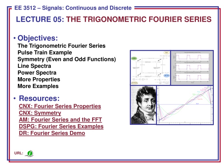
ECE 8443 Pattern Recognition EE 3512 Signals: Continuous and Discrete LECTURE 05: THE TRIGONOMETRIC FOURIER SERIES Objectives: The Trigonometric Fourier Series Pulse Train Example Symmetry (Even and Odd Functions) Line Spectra Power Spectra More Properties More Examples Resources: CNX: Fourier Series Properties CNX: Symmetry AM: Fourier Series and the FFT DSPG: Fourier Series Examples DR: Fourier Series Demo URL:
The Trigonometric Fourier Series Representations For real, periodic signals: = k or ( ) ( ) = + + ( ) cos sin " trigonomet ric Fourier series" x t a a k t b k t 0 0 0 k k 1 , = k = jk t ( ) " complex" x t c e 0 k The analysis equations for ak and bk are: 1 0 = T T ( ) a x t dt 0 T 2 T = = ( ) cos( ) , , 1 , 2 ... a x t k t dt k 0 k 0 T 2 T = = ( ) sin( ) , , 1 , 2 ... b x t k t dt k 0 k 0 Note that a0 represents the average, or DC, value of the signal. We can convert the trigonometric form to the complex form: 1 0 0 = = = c jb a c a c k k k k 1 + = ( ) ( ) , 1 , 2 ... a jb k k k 2 2 EE 3512: Lecture 05, Slide 1
Example: Periodic Pulse Train (Complex Fourier Series) T T 1 / 2 T ( ) jk t jk T jk T 1 1 1 1 e e e 1 0 0 1 0 1 = = = = jk t jk t ( ) ( ) c x t e dt x t e dt 0 0 k T T T jk T jk jk 0 0 0 / 2 T T T 1 1 jk T jk T 2 2 e e ( ) 0 1 0 1 = = k sin T 0 1 k sin 2 2 ( / ) T j k T T 0 ( ) k T = 0 1 k EE 3512: Lecture 05, Slide 2
Example: Periodic Pulse Train (Trig Fourier Series) T T / 2 T T 2 T 1 1 1 1 1 1 1 t = = = = = = 1 ( ) ( ) ) 1 ( ( ( )) a x t dt x t dt dt T T 0 1 1 T T T T T T T 0 / 2 T T 1 1 This is not surprising because a0 is the average value (2T1/T). Also, = a c sin 0 0 ( ) ( ) sin k T k T = = 0 1 0 1 c c 0 k k k = 0 k Use L' Hopital' s Rule : ( ( ) / sin ( ) cos( ) 2 ( / ) 2 k k T T k T T T T T = = = = = 0 ) 1 0 1 0 1 0 1 1 1 / k k T = 0 k = k 0 EE 3512: Lecture 05, Slide 3
Example: Periodic Pulse Train (Cont.) / 2 T / 2 T 2 2 T T = = ( ) cos( ) a x t k t dt ( ) sin( ) b x t k t dt 0 k 0 k T / 2 T / 2 T T T T 1 1 sin( ) cos( k ) k t k t 2 2 2 T 2 T 1 1 T = = = = 0 0 ( ) cos( ) ( ) sin( ) x t k t dt x t k t dt 0 0 T T k 0 0 T T T 1 1 1 1 = 0 sin( ) sin( ( )) k T k T 2 = 0 1 0 1 T 4 k k 0 0 sin( ) k T = 0 1 k T 0 Check this with our result for the complex Fourier series (k > 0): T 0 T 0 k 4 sin( ) 2 sin( ) sin( ) k T k T T 1 1 = = = = 0 1 0 1 0 1 ( ) ( ) 0 c a jb k k k k k k 2 2 EE 3512: Lecture 05, Slide 4
Even and Odd Functions 4 sin( ) k T = = 0 1 , 0 a b k k k T 0 Was this result surprising? Note: x(t) is an even function: x(t) = x(-t) = = T T T / 2 / 2 T T 2 2 ( ) cos( ) 2 ( ) cos( ) a x t k t dt x t k t dt 0 0 k / 2 0 / 2 T 2 T T = = ( ) sin( ) 0 b x t k t dt 0 k / 2 If x(t) is an odd function: x(t) = x(-t) / 2 T 2 T T = = ( ) cos( ) 0 a x t k t dt 0 k / 2 / 2 / 2 T T 2 T 2 T T = = ( ) sin( ) [ 2 ( ) sin( ) ] b x t k t dt x t k t dt 0 0 k / 2 0 EE 3512: Lecture 05, Slide 5
Line Spectra ( ) k sin T = 0 1 ck k 2 T = = ( ) 2 ( k ) k k k f 0 0 1 1 = = = + = Recall: ( ) ( ) , 1 , 2 ... c a c a jb c a jb k 0 0 k k k k k k 2 2 From this we can show: 1 1 = = + = 2 2 ( ) c a jb a b c k k k k k k 2 2 b 1 k tan 0 a k a b = = = 1 k k tan c c c k k k a b + 1 k k tan 0 a k a k EE 3512: Lecture 05, Slide 6
Energy and Power Spectra The energy of a CT signal is: = 2 ( ) E x t dt / 2 T 1 T T = 2 The power of a signal is defined as: ( ) P x t dt / 2 Think of this as the power of a voltage across a 1-ohm resistor. = k = jk t ( ) x t c ke Recall our expression for the signal: 0 We can derive an expression for the power in terms of the Fourier series coefficients: 2 / 2 / T k T T T 2 / 2 / 2 T T 1 1 1 = k = k 2 = = = = + + jk t 2 2 0 2 k 2 k ( ) P x t dt c e dt c a a b 0 k k 2 = 0 Hence we can also think of the line spectrum as a power spectral density: ( ) 2 k sin T 2 = 0 1 ck k EE 3512: Lecture 05, Slide 7
Properties of the Fourier Series x.JPG EE 3512: Lecture 05, Slide 8
Properties of the Fourier Series EE 3512: Lecture 05, Slide 9
Properties of the Fourier Series EE 3512: Lecture 05, Slide 10
Summary Reviewed the Trigonometric Fourier Series. Worked an example for a periodic pulse train. Analyzed the impact of symmetry on the Fourier series. Introduced the concept of a line spectrum. Discussed the relationship of the Fourier series coefficients to power. Introduced our first table of transform properties. Next: what do we do about non-periodic signals? EE 3512: Lecture 05, Slide 11


")
")
")


