Turbulence in Continuity Equation for Momentum
Explore the chaotic nature of turbulence in the solution of the continuity equation for momentum. Learn about the impact of pressure-gradient acceleration, inertial acceleration, viscous dissipation, and more. Delve into the transition from laminar to turbulent flow and the importance of subgrid scales in atmospheric dynamics.

Download Presentation

Please find below an Image/Link to download the presentation.
The content on the website is provided AS IS for your information and personal use only. It may not be sold, licensed, or shared on other websites without obtaining consent from the author. If you encounter any issues during the download, it is possible that the publisher has removed the file from their server.
You are allowed to download the files provided on this website for personal or commercial use, subject to the condition that they are used lawfully. All files are the property of their respective owners.
The content on the website is provided AS IS for your information and personal use only. It may not be sold, licensed, or shared on other websites without obtaining consent from the author.
E N D
Presentation Transcript
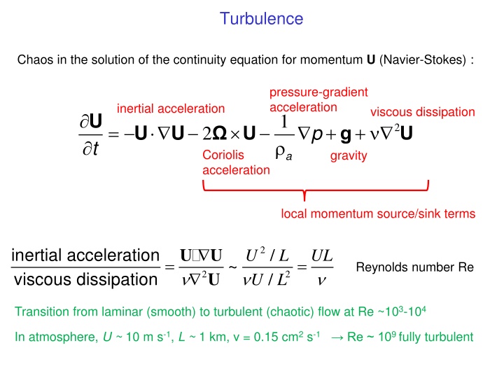
Turbulence Chaos in the solution of the continuity equation for momentum U (Navier-Stokes): pressure-gradient acceleration inertial acceleration viscous dissipation U t 1 = U + p + 2 U 2 Coriolis acceleration U g U gravity a local momentum source/sink terms 2 inertial acceleration viscous dissipation U U U / / U U L L UL = = ~ Reynolds number Re 2 2 Transition from laminar (smooth) to turbulent (chaotic) flow at Re ~103-104 In atmosphere, U ~ 10m s-1, L ~ 1 km, = 0.15 cm2 s-1 Re ~ 109 fully turbulent
Dealing with subgrid transport Atmospheric flow is turbulent down to mm scale where viscous dissipation (molecular diffusion) takes over Typical observations of surface wind (10 Hz) turbulent eddies Advection in models must cut off the subgrid scales: u = <u > + u instantaneous grid average fluctuating resolved unresolved (turbulent) deterministic stochastic Brasseur and Jacob, chap. 8.2
Importance of subgrid scales for mean transport CO2 Observations from Harvard Forest tower on a typical summer day (Bill Munger, Harvard) tower forest vertical wind w T CO2 w = <w> + w n = <n> + n n Time-averaged vertical flux <F> = <nw> = <n><w> + <n w > ... . resolved turbulent (small) (large) .... w Turbulent flux is covariance between fluctuating components . Brasseur and Jacob, chap. 10.2.4
Turbulent diffusion parameterization for small-scale eddies In 1-D (vertical) z z a F nw K n z resolved turbulent Compare to molecular diffusion D =0.1 cm2 s-1 implies Gaussian plumes for point sources Kz is empirical turbulent diffusion coefficient, same for all species (similarity assumption) Typical Kz ~ 105 cm2 s-1 C = California fire plumes, Oct 2004 Industrial plumes Generalized continuity equation in 3-D (Eulerian): K 0 0 0 x n t = + + n n C P L U K i = ( ) K K 0 0 with i a i i i y K 0 z Brasseur and Jacob, chap.8.4.1
Lagrangian treatment of small-scale eddies Treat turbulent component as Markov chain: = + 2 x u t K x x = + 2 y v t K y y position to+ t = w t + 2 z K z z where the random components have expected value of zero and standard deviation t ( ( x, y, z)T position to Brasseur and Jacob, chap. 4.11.2
Gaussian plume modeling of point source dispersion Point source with emission rate q Transport in cross-wind direction is parameterized as diffusive process: 2 2 C t C x C y C z = + + u K K for steady wind, inert plume y z 2 2 Turbulent diffusion coefficients Steady state solution with suitable boundary conditions: 2 2 q u y z K = + ( , , ) C x y z exp[ ( )] 4 ( 1/2 ) 4 K K x x K y z y z Brasseur and Jacob, chap. 4.12.1
Deep convection Subgrid in horizontal but organized in vertical very large eddy Requires non-local parameterization of mass transport Convective cloud (0.1-100 km) z detrainment C-shaped profile for species with surface source Model vertical levels Large-scale subsidence downdraft updraft entrainment C Model grid scale Brasseur and Jacob, chap. 8.8