Turbulent Flow Analysis on 2D Flat Plate: COMSOL Simulation
Explore a comprehensive study on the behavior of turbulent flows over a 2D flat plate using COMSOL simulations. This analysis delves into velocity and temperature profiles, turbulence models, wall functions, mesh resolution, and boundary layer thickness to validate theoretical predictions and computational approaches. Gain insights into the impact of wall treatments and mesh configurations on resolving sharp gradients near walls in turbulent flows.

Download Presentation

Please find below an Image/Link to download the presentation.
The content on the website is provided AS IS for your information and personal use only. It may not be sold, licensed, or shared on other websites without obtaining consent from the author. If you encounter any issues during the download, it is possible that the publisher has removed the file from their server.
You are allowed to download the files provided on this website for personal or commercial use, subject to the condition that they are used lawfully. All files are the property of their respective owners.
The content on the website is provided AS IS for your information and personal use only. It may not be sold, licensed, or shared on other websites without obtaining consent from the author.
E N D
Presentation Transcript
Background In turbulent flows, velocity and temperature profiles can be particularly sharp close to walls The high gradients require a fine mesh that is not always accessible in terms of computational cost Turbulence models and wall functions for both velocity and temperature aim at reducing this cost This zero pressure gradient 2D flat plate setup is part of a family of verification cases proposed by the NASA Langley Research Center Turbulence Modeling Resource (https://turbmodels.larc.nasa.gov) A wall-resolved and a wall-modeled approach are performed to attest the validity of velocity and temperature turbulence models and wall functions
Model Definition A 2D flat plate is placed in a turbulent flow at Mach number 0.2 and Reynolds number about 5 million The Algebraic y+ turbulence model is tested against theoretical velocity and temperature profiles The flow is nonisothermal and treated as compressible Model geometry Two studies are proposed, one considering only conduction and convection, and one with the addition of viscous dissipation in the heat transfer
Model Definition An inlet condition is set so that air enters the domain at 68 m/s and 300 K An open boundary is considered at the top, far enough to not interact with the boundary layer The no-slip wall is 2 m long, and is preceded by a symmetry condition A temperature condition of 301 K is set at the wall so that conduction fluxes exist between the fluid and the wall Model boundary conditions
Results The Algebraic y+ turbulence model comes with two possible wall treatments The Low Re one requires a fine mesh at the wall, typically with y+ values inferior to 1 at the first cell. It is used in this model to test the ability of the turbulence model to resolve the sharp velocity and temperature gradients at the wall The Automatic one works with both fine and coarser mesh, and is used here with y+ values superior to 30 at the first cell to test the ability of wall functions to model the unresolved contributions of sharp velocity and temperature gradients Mesh resolution and boundary layer thickness in the domain
Results When expressed in viscous units, the velocity profile in the boundary layer follows the law of the wall The wall-resolved approach is in good accordance with the theoretical velocity profile of the Algebraic y+ model in all sublayers (laminar, buffer, turbulent) The wall-modeled approach starts in the turbulent sublayer and fits really well with the wall-resolved approach The boundary layer ends at y+ about 10,000 where the velocity becomes constant, equals to the freestream velocity Velocity profiles in viscous units at x=0.97 m and x=1.9 m
Results The figure depicts the friction coefficient along the flat plate The wall-resolved and wall- modeled approaches are both in very good accordance The irregular perturbation at the beginning of the wall-resolved curve is due to the sudden change of velocity between the Symmetry and Wall boundary conditions Friction coefficient along the flat plate
Results The wall-resolved approach matches very well with the theoretical adimensional temperature In a conduction only case, the adimensional temperature resulting from the Standard wall function is close to the one from the wall-resolved study. The wall function slightly underestimates the wall heat flux, which explains the small difference The High viscous dissipation at wall wall function overestimates both the temperature in the boundary layer and the wall heat flux. It includes an additional source term for viscous dissipation at wall, which is not expected there as viscous dissipation is not included in this study Temperature profiles in viscous units at x=0.97 m and x=1.9 m
Results When viscous dissipation is accounted for and is not negligible, the High viscous dissipation at wall wall function is in good accordance with the wall- resolved approach The Standard wall function, which is not accounting for viscous dissipation, underestimates the temperature in the boundary layer Temperature profiles at x=0.97 m and x= 1.9m
Results Viscous dissipation is high in the boundary layer, especially very close to the wall in the laminar sublayer Resolving all the viscous dissipation requires a fine mesh, as shown with the wall-resolved approach The High viscous dissipation at wall wall function compensates the unresolved viscous dissipation with an additional source term in the heat transfer equation The Standard wall function does not account for viscous dissipation and is thus more relevant for studies where conduction is predominant Viscous dissipation profiles (Qvd) at x=0.97 m and x=1.9m