Two-Sample Problems & Comparing Population Means

A comprehensive overview of two-sample problems, comparing population means, and the application of t-procedures in statistical inference. Explore conditions for inference, standardization of differences, and the essence of independent samples. Understand the significance of estimating standard deviations and conducting permutation tests.

Download Presentation

Please find below an Image/Link to download the presentation.
The content on the website is provided AS IS for your information and personal use only. It may not be sold, licensed, or shared on other websites without obtaining consent from the author.If you encounter any issues during the download, it is possible that the publisher has removed the file from their server.
You are allowed to download the files provided on this website for personal or commercial use, subject to the condition that they are used lawfully. All files are the property of their respective owners.
The content on the website is provided AS IS for your information and personal use only. It may not be sold, licensed, or shared on other websites without obtaining consent from the author.
E N D
Presentation Transcript
Basic Practice of Statistics 7th Edition Lecture PowerPoint Slides
In Chapter 21, We Cover Two-sample problems Comparing two population means Two-sample t procedures Using technology Robustness again Details of the t approximation* Avoid the pooled two-sample t procedures* Avoid inference about standard deviations* Permutation tests*
Two-Sample Problems A two-sample problem can arise from a randomized comparative experiment that randomly divides subjects into two groups and exposes each group to a different treatment. Comparing random samples separately selected from two populations is also a two-sample problem. Unlike the matched pairs designs studied earlier, there is no matching of the individuals in the two samples. The two samples are assumed to be independent and can be of different sizes. The most common goal of inference is to compare the average or typical responses in the two populations.
Comparing Two Population Means CONDITIONS FOR INFERENCE COMPARING TWO MEANS We have two SRSs from two distinct populations. The samples are independent. That is, one sample has no influence on the other. We measure the same response variable for both samples. Both populations are Normally distributed. The means and standard deviations of the populations are unknown. In practice, it is enough that the distributions have similar shapes and that the data have no strong outliers. Call the variable ?1 in the first population and ?2 in the second because the variable may have different distributions in the two populations. Here is how we describe the two populations: Standard deviation Population Variable Mean ?1 ?1 ?1 1 ?2 ?2 ?2 2
Comparing Two Population Means Here is how we describe the two samples: Sample standard deviation Population Sample size Sample mean ?1 ?1 ?1 1 ?2 ?2 ?2 2 To do inference about the difference ?1 ?2 between the means of two populations, we start from the difference ?1 ?2 between the means of the two samples.
Two-Sample t Procedures To take variation into account, we would like to standardize the observed difference ?1 ?2 by subtracting its mean, ?1 ?2, and dividing the result by its standard deviation. This standard deviation of the difference in sample means is 2 2 ?1 ?1 +?2 ?2 Because we don't know the population standard deviations, we estimate them by the sample standard deviations from our two samples. The result is the standard error, or estimated standard deviation, of the difference in sample means: 2 2 ?1 ?1 +?2 ?? ?1 ?2= ?2
Two-Sample t Procedures When we standardize the estimate by subtracting its mean, ?1 ?2, and dividing the result by its standard error, the result is the two-sample t statistic: ?1 ?2 ?1 ?2 ? = 2 2 ?1 ?1+?2 ?2 The two-sample t statistic has approximately a t distribution. It does not have exactly a t distribution, even if the populations are both exactly Normal. In practice, however, the approximation is very accurate. There are two practical options for using the two-sample t procedures: Option 1. With software, use the statistic t with accurate critical values from the approximating t distribution. Option 2. Without software, use the statistic t with critical values from the t distribution with degrees of freedom equal to the smaller of ?1 1 and ?2 1. The significance test gives a P-value equal to or greater than the true P-value.
Two-Sample t Procedures THE TWO-SAMPLE t PROCEDURES Draw an SRS of size ?1 from a large Normal population with unknown mean ?1, and draw an independent SRS of size ?2 from another large Normal population with unknown mean ?2. A level Cconfidence interval for ?? ?? is given by 2 2 ?1 ?1 +?2 ?1 ?2 ? ?2 Here, ? is the critical value for confidence level C for the t distribution with degrees of freedom from either Option 1 (software) or Option 2 (the smaller of ?1 1 and ?2 1).
Two-Sample t Procedures THE TWO-SAMPLE t PROCEDURES To test the hypothesis ??: ?? = ??, calculate the two-sample t statistic: ?1 ?2 ? = 2 2 ?1 ?1+?2 ?2 Find P-values from the t distribution with degrees of freedom from either Option 1 (software) or Option 2 (the smaller of ?1 1 and ?2 1).
Example STATE: People gain weight when they take in more energy from food than they expend. James Levine and his collaborators at the Mayo Clinic investigated the link between obesity and energy spent on daily activity with data from a study with ?1= ?2= 10 health volunteers; 10 who were lean, 10 who were mildly obese but still healthy. They wanted to address the question: Do lean and obese people differ in the average time they spend standing and walking? PLAN: Give a 90% confidence interval for ?1 ?2, the difference in average daily minutes spent standing and walking between lean and mildly obese adults. SOLVE: Examination of the data reveals all conditions for inference can be (at least reasonably) assumed; the distributions are a bit irregular, but with only 10 observations this is to be expected.
Example SOLVE: (cont d) The descriptive statistics: Mean, ? ? Group Std. Dev., s 1 (lean) 10 525.751 107.121 2 (obese) 10 373.269 67.498 For using Option 2 (conservative degrees of freedom in absence of technology), ?1 1 = ?2 1 = 9, and t* = 1.833, giving: 107.1212 67.4982 2 2 ?1 ?1+?2 ?1 ?2 ? ?2= 525.751 373.269 1.833 + 10 10 = 152.482 73.390= 79.09 to 225.87 minutes Software using Option 1 gives df = 15.174 and t* = 1.752, for a confidence interval of 82.35 to 222.62 minutes narrower because Option 2 is conservative. CONCLUDE: Whichever interval we report, we are (at least) 90% confident that the mean difference in average daily minutes spent standing and walking between lean and mildly obese adults lies in this interval.
Example COMMUNITY SERVICE AND ATTACHMENT TO FRIENDS STATE: Do college students who have volunteered for community service work differ from those who have not? A study obtained data from 57 students who had done service work and 17 who had not. One of the response variables was a measure of attachment to friends. Here are the results: ? ? Group Condition s 1 Service 57 105.32 14.68 2 No service 17 96.82 14.26 PLAN: The investigator had no specific direction for the difference in mind before looking at the data, so the alternative is two-sided. We will test the following hypotheses: ?0:?1= ?2 ??:?1 ?2
Example SOLVE: The two-sample t statistic: ?1 ?2 ? = 2 2 ?1 ?1+?2 ?2 105.32 96.82 = 14.682 57 8.53.9677= 2.142 +14.262 17 = Software (Option 1) says that the two-sided P-value is 0.0414. For using Option 2, ?1 1 = 56, ?2 1 = 16, and therefore comparing our test statistic of 2.142 to two-sided critical values of a t(16) distribution, Table C shows the P-value is between 0.05 and 0.04. CONCLUDE: The data give moderately strong evidence (P < 0.05) that students who have engaged in community service are, on the average, more attached to their friends.
Using Technology CrunchIt and the calculator get Option 1 completely right. The accurate approximation uses the t distribution with approximately 15.174 (CrunchIt rounds this to 15.17) degrees of freedom. The P-value is P = 0:0008.
Using Technology Minitab uses Option 1, but it truncates the exact degrees of freedom to the next smaller whole number to get critical values and P-values. In this example, the exact df = 15.174 is truncated to df = 15 so that Minitab's results are slightly conservative. That is, Minitab's P-value (rounded to P = 0:001 in the output) is slightly larger than the full Option 1 P-value. Excel rounds the exact degrees of freedom to the nearest whole number so that df = 15.174 becomes df = 15. Excel s method agrees with Minitab s in this example. But when rounding moves the degrees of freedom up to the next higher whole number, Excel s P-values are slightly smaller than is correct. This is misleading, another illustration of the fact that Excel is substandard as statistical software.
Robustness Again The two-sample t procedures are more robust than the one-sample t methods, particularly when the distributions are not symmetric. When the sizes of the two samples are equal and the two populations being compared have distributions with similar shapes, probability values from the t table are quite accurate for a broad range of distributions when the sample sizes are as small as ?1= ?2= 5. When the two population distributions have different shapes, larger samples are needed. As a guide to practice, adapt the guidelines for one-sample t procedures to two-sample procedures by replacing sample size with the sum of the sample sizes, ?1+ ?2. Caution: In planning a two-sample study, choose equal sample sizes whenever possible. The two-sample t procedures are most robust against non-Normality in this case, and the conservative Option 2 probability values are most accurate.
Details of the t Approximation* The exact distribution of the two-sample t statistic is not a t distribution. The distribution changes as the unknown population standard deviations change. However, an excellent approximation is available. APPROXIMATE DISTRIBUTION OF THE TWO-SAMPLE t STATISTIC The distribution of the two-sample t statistic is very close to the t distribution with degrees of freedom given by 2 2 2 ?1 ?1+?2 2 + ?2 ?? = 2 2 2 ?2 ?2 ?1 ?1 1 1 ?1 1 ?2 1 This approximation is accurate when both sample sizes ?1 and ?2 are 5 or larger.
Avoid the Pooled Two-Sample t Procedures* Many calculators and software packages offer a choice of two-sample t statistics. One is often labeled for unequal variances; the other for equal variances. The unequal variance procedure is our two-sample t. Never use the pooled t procedures if you have software or technology that will implement the unequal variance procedure.
Avoid Inference About Standard Deviations* There are methods for inference about the standard deviations of Normal populations. The most common such method is the Ftest for comparing the standard deviations of two Normal populations. Unlike the t procedures for means, the F test for standard deviations is extremely sensitive to non- Normal distributions. We do not recommend trying to do inference about population standard deviations in basic statistical practice.
Permutation Tests* As an alternative to two-sample t tests, in some instances it may be to our advantage to perform a permutation test in general, if experimental units are assigned to two treatment groups completely at random, and our null hypothesis is no treatment effect, we can test hypotheses using sample means as follows: First, list all possible ways units can be assigned to treatment groups. Second, based on the data obtained, for each possible assignment determine what the difference in means (mean for treatment 1 minus mean for treatment 2) would be. Under the null hypothesis, each of these is equally likely.
Permutation Tests* Permutation test method (cont d): Third, determine the distribution of these possible outcomes by listing all the different possible mean differences and their corresponding probabilities (this can also be represented by a histogram). Using this sampling distribution, determine the P-value of the actual mean difference you obtained. The resulting sampling distribution of outcomes is called the permutation distribution. Practical issues: First: Unless the number of ways units can be assigned is sufficiently large, the smallest possible P-value may not be very small. Second: Listing all possible outcomes can be tedious Third: Permutation method is most likely to be useful with small- to moderate-size experiments because of the robustness of t procedures.