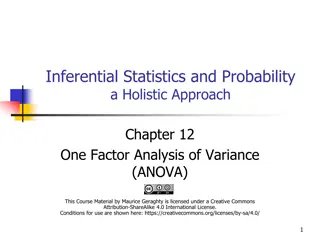
Understanding ANOVA in Social Statistics

Social Statistics: ANOVA

Review 2

The problem with t-tests How to compare the difference on >2 groups on one or more variables If it is only one variable, we could compare three groups with multiple ttests: M1 vs. M2, M1 vs. M3, M2 vs. M3 >2 variables? For example, how two teaching methods are different for three different sizes of classes. ANOVA allows you to see if there is any difference between groups on some variables. 3

What is ANOVA? Analysis of Variance A hypothesis-testing procedure used to evaluate mean differences between two or more treatments (or populations) on different variables. ANOVA is available for both parametric (score data) and non-parametric (ranking) data. Advantages: 1) Can work with more than two samples. 2) Can work with more than one independent variable 4

One example Assume that you have data on student performance in non-assessed tutorial exercises as well as their final grading. You are interested in seeing if tutorial performance is related to final grade. ANOVA allows you to break up the group according to the grade and then see if performance is different across these grades. 5

Types of ANOVA? One-way between groups Differences between the groups The groups are categorized in one way, such as groups were divided by age, or grade. This is the simplest version of ANOVA It allows us to compare variable between different groups, for example, to compare tutorial performance from different students grouped by grade. 6

Types of ANOVA? One-way repeated measures A single group has been measured by a variable for a few times Example 1: one group of patients were tested by a new drug in different times: before taking the drug, after taking the drug Example 2: student performance on the tutorial over time. 7

Types of ANOVA? Two-way between groups For example: the grades by tutorial analysis could be extended to see if overseas students performed differently to local students. What you would have from this form of ANOVA is: The effect of final grade The effect of overseas versus local The interaction between final grade and overseas/local Each of the main effects are one-way tests. The interaction effect is simply asking "is there any significant difference in performance when you take final grade and overseas/local acting together". 8

Types of ANOVA? Two-way repeated measures Use the repeated measures Include an interaction effect For example, we want to see the performance of tutorial about gender and time of testing. We have the same two groups (male, and female groups) and test them in different times to compare the difference. 9

What is ANOVA? In ANOVA an independent or quasi- independent variable is called a factor. Factor = independent (or quasi-independent) variable. Levels = number of values used for the independent variable. One factor single-factor design More than one factor factorial design 10

What is ANOVA? An example of a single-factor design A example of a two-factor design 11

How ANOVA works? ANOVA calculates the mean for each of the final grading groups on the tutorial exercise figure - the Group Means. It calculates the mean for all the groups combined - the Overall Mean. Then it calculates, within each group, the total deviation of each individual's score from the Group Mean - Within Group Variation. Next, it calculates the deviation of each Group Mean from the Overall Mean - Between Group Variation. Finally, ANOVA produces the F statistic which is the ratio Between Group Variation to the Within Group Variation. If the Between Group Variation is significantly greater than the Within Group Variation, then it is likely that there is a statistically significant difference between the groups. The statistical package will tell you if the F ratio is significant or not. All versions of ANOVA follow these basic principles but the sources of Variation get more complex as the number of groups and the interaction effects increase. 12

F value Variance between treatments can have two interpretations: Variance is due to differences between treatments. Variance is due to chance alone. This may be due to individual differences or experimental error. 13

Excel: ANOVA Data Analysis Analysis Tools three different ANOVA: Anova: Single Factor (one-way between groups) Anova: Two-factors With Replication Anova: Two-Factors Without Replication 14

Example (one-way ANOVA) Three groups of preschoolers and their language scores, whether they are overall different? Group 1 Scores 87 86 76 56 78 98 77 66 75 67 Group 2 Scores 87 85 99 85 79 81 82 78 85 91 Group 3 Scores 89 91 96 87 89 90 89 96 96 93 15

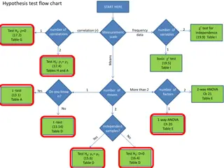
F test steps Step1: a statement of the null and research hypothesis One-tailed or two-tailed (there is no such thing in ANOVA) = = 0: H 1 2 3 different is least at : one H 1 16

F test steps Step2: Setting the level of risk (or the level of significance or Type I error) associated with the null hypothesis 0.05 17

F test steps Step3: Selection of the appropriate test statistics Groups Count 1 10 2 10 3 10 Sum Average Variance 766 852 916 76.6 143.1556 85.2 91.6 38.4 11.6 ANOVA: Single factor 18

F test steps Group 1 Scores x square Group 2 Scores x square Group 3 Scores x square 87 86 76 56 78 98 77 66 75 67 7569 7396 5776 3136 6084 9604 5929 4356 5625 4489 87 85 99 85 79 81 82 78 85 91 7569 7225 9801 7225 6241 6561 6724 6084 7225 8281 89 91 96 87 89 90 89 96 96 93 7921 8281 9216 7569 7921 8100 7921 9216 9216 8649 n x 10 766 10 852 10 916 N X ( ( 30 2534 2 ) 2) ) / X N X X ( 76.6 85.2 91.6 214038.5333 2 ( ) 2 (X X 59964 58675.6 72936 72590.4 84010 83905.6 216910 215171.6 2 ) / / X n n

F-test Between sum of squares within sum of squares total sum of squares X 2 2 ( ) / ( ) / X n X N 215171.6-214038.53 1133.07 2 2 ( ) ( ) / X n 216910-215171.60 1738.40 2 2 ( ) ( ) / X X N 216910-214038.53 2871.47

F test steps Between-group degree of freedom=k-1 k: number of groups Within-group degree of freedom=N-k N: total sample size sums of squares mean sums of squares source df F Between groups 1133.07 2 566.53 8.799 Within gruops 1738.40 27 64.39 Total 2871.47 29

F test steps Between-group degree of freedom=k-1 k: number of groups Within-group degree of freedom=N-k N: total sample size 22

F test steps Step4: (cont.) df for the denominator = n-k=30-3=27 df for the numerator = k-1=3-1=2 23

F test steps Step4: determination of the value needed for rejection of the null hypothesis using the appropriate table of critical values for the particular statistic Table-Distribution of F (http://www.socr.ucla.edu/applets.dir/f_table.html) 24

F test steps Step5: comparison of the obtained value and the critical value If obtained value > the critical value, reject the null hypothesis If obtained value < the critical value, accept the null hypothesis 8.80 and 3.36 25

F test steps Step6 and 7: decision time What is your conclusion? Why? How do you interpret F(2, 27)=8.80, p<0.05 26