Understanding Back-Propagation in Neural Networks
Learn about back-propagation, a key concept in neural networks for optimizing performance. Explore flow diagrams, gradient descent, and the chain rule of calculus. Dive into how neural networks calculate computations, adjust parameters, and optimize outputs through back-propagation.

Download Presentation

Please find below an Image/Link to download the presentation.
The content on the website is provided AS IS for your information and personal use only. It may not be sold, licensed, or shared on other websites without obtaining consent from the author. If you encounter any issues during the download, it is possible that the publisher has removed the file from their server.
You are allowed to download the files provided on this website for personal or commercial use, subject to the condition that they are used lawfully. All files are the property of their respective owners.
The content on the website is provided AS IS for your information and personal use only. It may not be sold, licensed, or shared on other websites without obtaining consent from the author.
E N D
Presentation Transcript
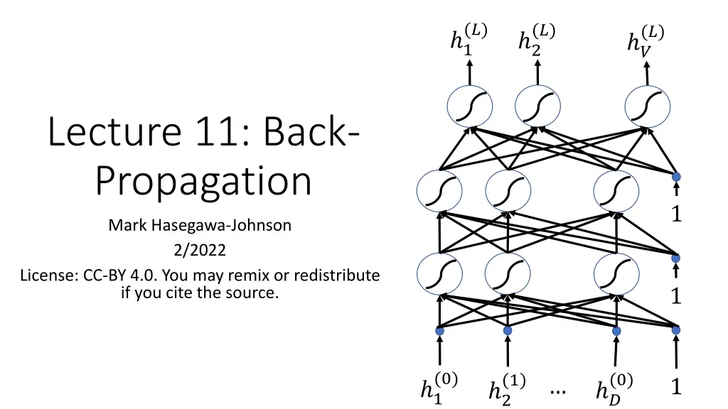
(?) (?) (?) 1 2 ? Lecture 11: Back- Propagation 1 Mark Hasegawa-Johnson 2/2022 License: CC-BY 4.0. You may remix or redistribute if you cite the source. 1 (0) (0) (1) 1 1 ? 2
Outline Review: flow diagrams Gradient descent The chain rule of calculus Back-propagation
Flow diagrams A flow diagram is a way to represent the computations performed by a neural network. Circles, a.k.a. nodes, a.k.a. neurons, represent scalar operations. The circles above ?1 and ?2 represent the scalar operation of read this datum in from the dataset. The circles labeled 1 and 1 represent the scalar operation of unit step function. Lines represent multiplication by a scalar. Where arrowheads come together, the corresponding variables are added. ? 0.5 1 1 1 2 1.5 1 1 1 1 0.5 ?2 ?1 1
Flow diagrams Usually, a flow diagram shows only the activations (including inputs). Excitations, weights, biases, and nonlinearities are implicit. For example, this flow diagram means that there are some nonlinearities ?(?), and some weights ??,? 1= ?(1)?1 2= ?(1)?2 ? = ?(2)?1 ? 1 2 (?)and biases ?? (1)+ ?1,1 (1)+ ?2,1 (2)+ ?1 (?)such that: (1)?1+ ?1,2 (1)?1+ ?2,2 (2) 1+ ?2 (1)?2 (1)?2 (2) 2 ?1 ?2
Flow diagrams The important piece of information shown in a flow diagram is the order of computation. This flow diagram shows that, given ?1 and ?2, First, you calculate 1 and 2, then you can calculate ?. ? 1 2 ?1 ?2
Outline Review: flow diagrams Gradient descent The chain rule of calculus Back-propagation
Gradient descent: basic idea Suppose we have a training token, ?. Its target label is ?. The neural net produces output ?(?), which is not ?. The difference between ? and ?(?) is summarized by some loss function, (?,?(?)). The output of the neural net is determined by some parameters, ??,? Then we can improve the network by setting: (?). ? (?) ??,? (?) ? ??,? (?) ???,?
Gradient descent in a multi-layer neural net Just like in linear regression, the MSE loss is still a quadratic function of ?( ?) : =1 ? ?=1 but now, ?( ?) is a complicated nonlinear function of the weights. Therefore, if we draw (?), it s no longer a simple parabola. ? 2 ?( ??) ?? ?
Gradient descent in a multi-layer neural net Even though (?) is complicated, we can still minimize it using gradient descent: ? ? ? ? ?
Visualizing gradient descent https://cs.stanford.edu/people/karpathy/convnetjs/demo/classify2d.html
Outline Review: flow diagrams Gradient descent The chain rule of calculus Back-propagation
Definition of gradient ? The gradient is the vector of partial derivatives: ? ? (2) (2) 2 1 (1) ??1,1 ? ? (1) (1) ? = 1 2 (1) ??1,2 (1) ?1,2 ? ? (3) ?1 ??1,2 ?2
Definition of partial derivative ? The partial derivative of ? with respect to ?1,2 change ?1,2 all of the other weights the same. If we define ?1,2 the ?1,2 else, then: ? + ? ?1,2 (1)is what we get if we (1)to ?1,2 (2) (2) (1)+ ?, while keeping 2 1 1 to be a vector that has a 1 in (1) place, and zeros everywhere (1) (1) 1 2 (1) ?1,2 1 ? ? ? = lim ? 0 (1) ? ??1,2 ?1 ?2
Lots of different partial derivatives ? There are a lot of useful partial derivatives we could compute. For example: (2) (2) 2 1 ? (2) is the partial derivative of with (2) ? 1 respect to 1 (2), while keeping all other (1) (1) (2) 1 2 1 2 (1) ?1,2 elements of the vector (2)= (2) constant. ?1 ?2
The chain rule of calculus ? depends on ?, which depends on ?1,2 We can calculate ? ? (1). (2) (2) 2 1 (1) by chaining ??1,2 (multiplying) the two partial derivatives along the flow path: (1) (1) 1 2 (1) ?1,2 ? ? =? ?? ?? ? ??1,2 (1) (1) ??1,2 ?1 ?2
More chain rule ? (1), which depends on ? depends on 1 ?1,2 We can calculate ?? ? (1). (2) (2) 2 1 (1)by chaining: ??1,2 (1)? (1) ?? ?? (1) (1) (1) ? ? =? ? 1 1 2 (1) ?1,2 (1) (1) ??1,2 ? 1 ??1,2 ?1 ?2
More chain rule ? (2) and 2 (1). (2). Both 1 (2) and 2 (2) ? depends on 1 depend on 1 To apply the chain rule here, we need to sum over both of the flow paths: (2) (2) 2 1 2 1 ?? ?? 2 1 ? 1 ? ? =? ? 1 ? (1) (1) 1 2 (1) (1) 2 1 1 ??1,2 ? 1 ? 1 ??1,2 (1)? (1) ?1,2 (2) (1) (1) ?? ?? (2) ? 2 +? ? 1 (2) ? 2 ? 1 ??1,2 ?1 ?2
Outline Review: flow diagrams Gradient descent The chain rule of calculus Back-propagation
Back-propagation ? The key idea of back-propagation is to calculate ? ? ???,? pair of nodes j and k, as follows: Start at the output node. Apply the chain rule of calculus backward, layer-by-layer, from the output node backward toward the input. (?), for every layer l, for every (2) (2) 2 1 (1) (1) 1 2 (1) ?1,2 ?1 ?2
Back-propagation ? First, calculate ? ??. (2) (2) 2 1 (1) (1) 1 2 (1) ?1,2 ?1 ?2
Back-propagation ? First, calculate ? ??. Second, calculate (2) (2) 2 1 ? 2 ?? ?? 2 =? (2) 2 ? 1 ? 1 and (1) (1) 1 2 ? 2 ?? ?? 2 (1) =? ?1,2 (2) 2 ? 2 ? 2 ?1 ?2
Back-propagation ? Third, calculate ? 1 (1) (2) 1 ? 2 ? ? = (2) (2) (2) 2 1 1 ? 1 ? ? ? 1 ? and ? 1 (2) 1 ? 2 ? ? (1) = (1) 1 2 (1) (2) 1 (1) ? 2 ? ? ? 2 ?1,2 ? ?1 ?2
Back-propagation ? Fourth, calculate (1)? ? 1 ? ? ? ? = (2) (2) (1) (1) (1) 2 1 ??1,2 ? ? ??1,2 ? (1) (1) 1 2 (1) ?1,2 ?1 ?2
Back-propagation: splitting it up into excitation and activation Activation to excitation: here, the derivative is pre-computed. For example, if g=ReLU, then g =unit step: ? ? ? (?)= ReLU ?? (?) (?) ? ?= ? ?? ??? Excitation to activation: here, the derivative is just the network weight! ? ??? (? 1)= ??,? (?)= ?? (?)+ (?) ? (? 1) (?) ?? ??,? ? ? ?
Back-propagation: splitting it up into excitation and activation Excitation to network weight: here, the derivative is the previous layer s activation: ? ??? (?)= ?? (?)+ (?) ? (? 1) (? 1) ?? ??,? (?)= ? ???,? ?
? Finding the derivative Loss ? (3) ? (3) ? ? Forward propagate, from ?, to find ? Back-propagate, from ?, to find (? 1) in each layer Layer 3 ? (?) ? (2) ? ? ? (2) ? ? in each layer Multiply them to get ? (?), then Layer 2 ???? ? (1) ? (1) ? ? ? (?) ??? (?) ? ??? (?) ???? Layer 1 ?
Outline Review: flow diagrams Gradient descent ? ? ? ? The chain rule of calculus (2) 1 ? 1 ? 2 ? ? = (1) (2) 1 ? 2 ? ? ? 2 ? Back-propagation Apply the chain rule of calculus backward, layer-by-layer, from the output node backward toward the input.
")


