Understanding BCS Theory: Self-Consistent Solutions and Quasiparticles

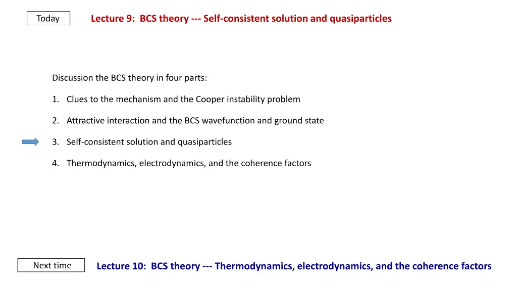
Lecture 9: BCS theory --- Self-consistent solution and quasiparticles Today Discussion the BCS theory in four parts: 1. Clues to the mechanism and the Cooper instability problem 2. Attractive interaction and the BCS wavefunction and ground state 3. Self-consistent solution and quasiparticles 4. Thermodynamics, electrodynamics, and the coherence factors Next time Lecture 10: BCS theory --- Thermodynamics, electrodynamics, and the coherence factors

Last time ( ) + + = + 0 u k k v c c BCS ground state: G k k 1,... k k m 2 = probability that the pair state (?, ?) is occupied ?? 2+ ?? 2= 1 ?? 2 = probability that the pair state (?, ?) is empty ?? 1 2 k k c c + + + = + H V c c c c BCS (reduced) H: R k k k k , k k = E H to determine the ground state Variational calculation to minimize BCS G R G 11 2 = + 2 k = + u k 2 k 2 k E Found where k E k = 11 2 k V u v = 2 k v k and k E k Today Diagonalize HR excitation spectrum

Self-Consistent solutions = b c c : Key feature of the BCS state is electron correlations In the normal state these vanish (phases are random) k k k average ( ) = + + k b = c c c c b b k k k k k k k instantaneous time- averaged deviation (assume fluctuations small) ( )( ) + + + = + H c c V c c c c R k k k k k k k k ( ) + + + = + + * k * k k 2 c c V c c b b c c b b neglect terms of k k k k k k k k = k V k V b Define k to absorb parameter This is the model Hamiltonian: bilinear in ( k c c ( ) + + + ) = + * k * H c c c c c c k k b + + ( ) c c M k k k k and k k k k k k k ( ) H H H Diagonalize by a linear canonical transformation model red * kb Is to be determined self-consistently after we find the ground state

Bogoliubov-Valatin Transformation + + = + * k v c u 0 1 k k k k + + = + * k v c u 1 0 k k k k + + = + ' c k + c k v v + ks u --- obey anti-commutation relations Fermi operators 0 k k k INVERT 0,1 + = c c k u spin degrees of freedom (mix electron spins) 1 k k k k ( ) + + + = + * k * H c c c c c c k k b M k k k k k k k k + + + , Want to get rid of product states and keep only terms of form 1 0 1 0 k k k k + = * k k v 2 2 k 2 0 u v u Diagonalization condition: k k k k ( ) + + = + + + * ( ) H E k k b E Leads to: 0 0 1 1 M k k k k k k k k k

Solve diagonalization condition to get ground state + = * k k v 2 2 k 2 0 u v u k k k k 2 * k * k k v u * k k v u 2 + = 2 0 Multiply by k k 2 k u k k 2 + 2 k 2 4 4 * k k v u Solve by quadradic formula: = + + = 2 2 k k E = k k k k k (+ solution is stable) 2 k * k k v u u v , , Phases of related: for energy to be real, must be real k k k k real , v u BCS chose have the same phase factor k k k = v e u u = i ke v = i k k k k k 11 2 11 2 2 2 = = + = + 2 2 v k u k Solution: E k k k k k E E k k

( ) ( ) + + = + + + * H E k k b E Result of the diagonalization: 0 0 1 1 M k k k k k k k k k ( ) = = 2 E First term: Normal State k k k N k k k F 2 ( ) 1 + 2 k 2 k 2 Superconducting State k V k KE PE 1 2N ( ) 0 = 2 DIFFERENCE Ground state Condensation energy E = excitation energy, Second term: excitation numbers of Bogoliubov quasiparticles k Self consistency = E k V c c k k av energy gap + + = * 1 V u v k 0 0 1 1 k ave = k No ' as before qp s V u v k k

Quasiparticle operators ( ) , 0 1 k k + + = u c v c 0 k k k k + k + = + u c v c 1 k k k k k 0 0 = = 0 ( ) Define ground state by: ( ) 0 k G + + + + + e.g. c 0 u c v u v c c k k 0 k k 1 k G ( )0 ( ) + + + + = 0 u v u v c u v c c k k k k k k 0 0 + ( ) Define quasiparticle by: ( ) 0 k G + + + + e.g. 0 u c v c u v c c + k k k k k 1 k G ( ) ( ) + + + + + 2 k 2 k 0 u v c u v c c k k k k k k + state occupied, empty rest are unchanged from GS k k ko G ( )0 + + + + c u v c c k k k k k + state occupied, empty k k k 1 k G

Normal state Excitation picture describe excited states by addition of quasi-particles EXCITATIONS GROUNDSTATE OCCUPATION PROBABLILITY k + c 1 = N F k + k k k F k c k + k T 1 e B k c c k k k F kf k k E k = holes electrons 0 E ENERGY: k k k = Q e k 0 CHARGE: k k Q k 1 k = = V E v k VELOCITY: k k k k e k k 0 = = J ev Q V e CURRENT: k k k k

SUPERCONDUCTING STATE OCCUPATION PROBABILITY EXCITATIONS GROUND STATE 1 k T k + = F 0 k + E 1 e k B k k k 1 1 2 k k 2 kv k k E minimum excitation energy = + 2 k 2 E Energy: k k 0 2 k ( ) kE KE = = 1 2 = 2 k 2 k 2 v v k k k E k 2 k 2 k electron ground state = + = E E KE k E E 2 k k k ( ) PE = = 2 (lose pairing) u v PE k k k E k

electron GS ( ) = 1 2 = 2 k Q v e e k Charge: k E k Q k electron like qp s k Dependence of charge on means the qp changes charge as it accelerates k qp s not independent particles (many body system.) hole-like qp s k k 1 = = VELOCITY: V E v k k k k k E k Again, shows that qp s are not independent of condensate. = = CURRENT: J ev Q V ev k k k k k k E k QP s have mixed electron hole character

E Density of states: map over k k ( ) ( ) ( ) 0 = N E dE N d N d s k k N k k k d dE ( ) E ( ) 0 = k N N s k 0 E E E = N N = s ( ) E E s N 1/2 2 2 E N States below gap (NORMAL STATE) pushed up to peak at gap edge E Tunneling and transport are probes of this.

BCS Model GROUND STATE 1 2 E ( ) 0 11 2 = 2 c E N = + 2 k 2 k F = E 2 k k v k E k Self-consistency: , k E QUASIPARTICLES k mp ( ) T = = k Q e J ev Q V = k V v k k k k k k k E E k k cT E T for E ( ) N E = 2 2 E Next time: 0 for E Temperature dependence 1 k T ( ) = F E k + / E Thermodynamics phenomenological models 1 e k B External perturbations coherence factors (selection, modes)