Understanding Binomial Distribution in Probability Theory
Explore the concept of binomial distribution in probability theory, covering topics such as Bernoulli trials, Bernoulli process, and calculating the probability distribution of successes in a series of trials. Dive into examples to understand how to apply binomial distribution in real-world scenarios.

Download Presentation

Please find below an Image/Link to download the presentation.
The content on the website is provided AS IS for your information and personal use only. It may not be sold, licensed, or shared on other websites without obtaining consent from the author. If you encounter any issues during the download, it is possible that the publisher has removed the file from their server.
You are allowed to download the files provided on this website for personal or commercial use, subject to the condition that they are used lawfully. All files are the property of their respective owners.
The content on the website is provided AS IS for your information and personal use only. It may not be sold, licensed, or shared on other websites without obtaining consent from the author.
E N D
Presentation Transcript
Discrete Probability ristu.saptono@staff.uns.ac.id
Outline Binomial Distribution Poisson Distribution
Bernoulli Trial Bernoulli outcomes. The two possible outcomes are labeled: success (s) and failure (f) The probability of success is P(s)=p and the probability of failure is P(f)= q = 1 p. Examples: Tossing a coin (success=H, failure=T, and p=P(H)) Inspecting an item (success=defective, failure=non- defective, and p=P(defective)) trial is an experiment with only two possible
Bernoulli Process Bernoulli process is an experiment that must satisfy the following properties: The experiment consists of n repeated Bernoulli trials. The probability of success, P(s)=p, remains constant from to trial. The repeated trials are independent; that is the outcome of one trial has no effect on the outcome of any other trial trial
Consider the random variable : X = The number of successes in the n trials in a Bernoulli process The random variable X has parameters n (number of trials) and p (probability of success), and we write: X ~ Binomial(n,p) or X~b(x;n,p) a binomial distribution with
The probability distribution of X is given by: n x n x 0 = 1 ( ) ; , 1 , 0 , 2 , p p x n = = = = ( ) ( ) ( ; , ) f x P X x b x n p x ; otherwise
We can write the probability distribution of X as a table as follows. x f(x)=P(X=x)=b(x;n,p) n 0 n 0 ( ) ( )n 0 n 0 = 1 1 p p p 1 ( ) 1 n 11 p p 1 n 2 ( ) n 2 2 p 1 p 2 n n 1 ( )1 11 n p p 1 n n n ( ) 0 n n = 1 p p p n Total 1.00
Example Suppose that 25% of the products of a manufacturing process are defective. Three items are selected at random, inspected, and classified as defective (D) or non-defective (N). Find the probability distribution of the number of defective items. Solution Experiment: selecting 3 items at random, inspected, and classified as (D) or (N). The sample space is S={DDD,DDN,DND,DNN,NDD,NDN,NND,NNN} Let X = the number of defective items in the sample We need to find the probability distribution of X.
Outcome Probability X 3 3 3 27 NNN 0 First Solution = 4 3 4 3 4 1 64 9 NND 1 = 4 3 4 1 4 3 64 9 NDN 1 = 4 3 4 1 4 1 64 3 NDD 2 = 4 1 4 3 4 3 64 9 DNN 1 = 4 1 4 3 4 1 64 3 DND 2 = 4 1 4 1 4 3 64 3 DDN 2 = 4 4 4 64 1 1 1 1 DDD 3 = 4 4 4 64
The probability distribution .of X is x f(x)=P(X=x) 27 0 64 9 9 9 27 1 + + = 64 3 64 3 64 3 64 9 2 + + = 64 64 1 64 64 3 64
Second Solution Bernoulli trial is the process of inspecting the item. The results are success=D or failure=N, with probability of success P(s)=25/100=1/4=0.25. The experiments is a Bernoulli process with:
number of trials: n=3 Probability of success: p=1/4=0.25 X ~ Binomial(n,p)=Binomial(3,1/4) The probability distribution of X is given by: = = = = x b x X P ) 4 3 1 3 3 x x 0 ; = ( ) ( ) ; , 1 , 0 3 , 2 x 1 ( ) ( ) ( , 3 ; f x 4 4 x otherwise 3 The probability distribution of X is 1 1 3 27 0 3 = = = = = ) 0 ( ( ) 0 , 3 ; 0 ( b ) ( ) ( ) f P X 0 3 4 1 4 1 4 3 64 9 x f(x)=P(X=x) =b(x;3,1/4) 27/64 27/64 9/64 1/64 2 1 3 = = = = = ) 2 ( ( ) 2 , 3 ; 2 ( b ) ( ) ( ) f P X 2 4 4 4 64 1 0 1 2 3 1 1 3 3 0 = = = = = ) 3 ( ( ) 3 , 3 ; 3 ( b ) ( ) ( ) f P X 3 4 4 4 64
Theorem The mean and the variance of the binomial distribution b(x;n,p) are: = n p 2 = n p (1 p)
Example: In the previous example, find the expected value (mean) and the variance of the number of defective items. Suppose that 25% of the products of a manufacturing process are defective. Three items are selected at random, inspected, and classified as defective (D) or non-defective (N). Find the probability distribution of the number of defective items.
Solution: X = number of defective items We need to find E(X)= and Var(X)= 2 We found that X ~ Binomial(n,p)=Binomial(3,1/4) .n=3 and p=1/4 The expected number of defective items is E(X)= = n p = (3) (1/4) = 3/4 = 0.75 The variance of the number of defective items is Var(X)= 2 = n p (1 p) = (3) (1/4) (3/4) = 9/16 = 0.5625V
Example: In the previous example, find the following probabilities: (1) The probability of getting at least two defective items. (2) The probability of getting at most two defective items. Solution: X ~ Binomial(3,1/4) 3 1 3 3 x x 0 = ( ) ( ) , 0 , 1 3 , 2 for x 1 = = = = ( ) ( ) ( , 3 ; ) f x P X x b x 4 4 x 4 otherwise x .f(x)=P(X=x)=b(x;3,1/4) 0 27/64 1 27/64 2 9/64 3 1/64
(1) The probability of getting at least two defective items: 9 1 10 P(X 2)=P(X=2)+P(X=3)= f(2)+f(3)= + = 64 64 64 (2) The probability of getting at most two defective item: P(X 2) = P(X=0)+P(X=1)+P(X=2) 27 27 9 63 + + = = f(0)+f(1)+f(2) = 64 64 64 64 or P(X 2)= 1 P(X>2) = 1 P(X=3) = 1 f(3) = 1 63 = 1 64 64
Poisson Probability Distribution The Poisson distribution can be described mathematically using the formula: 20
Poisson Probability Distribution The mean number of successes can be determined in binomial situations by n , where n is the number of trials and the probability of a success. The variance of the Poisson distribution is also equal to n . 21
Poisson Probability Distribution - Example Assume baggage is rarely lost by Northwest Airlines. Suppose a random sample of 1,000 flights shows a total of 300 bags were lost. Thus, the arithmetic mean number of lost bags per flight is 0.3 (300/1,000). If the number of lost bags per flight follows a Poisson distribution with u = 0.3, find the probability of not losing any bags. 22
Poisson Probability Distribution - Example Assume baggage is rarely lost by Northwest Airlines. Suppose a random sample of 1,000 flights shows a total of 300 bags were lost. Thus, the arithmetic mean number of lost bags per flight is 0.3 (300/1,000). If the number of lost bags per flight follows a Poisson distribution with u = 0.3, find the probability of not losing any bags. 23
Example Arrivals at a bus-stop follow a Poisson distribution with an average of 4.5 every quarter of an hour. Obtain a barplot of the distribution (assume a maximum of 20 arrivals in a quarter of an hour) and calculate the probability of fewer than 3 arrivals in a quarter of an hour.
The probabilities of 0 up to 2 arrivals can be calculated directly from the formula x e with =4.5 = ( ) p x ! x 4.5 0 4.5 0! e = (0) p So p(0) = 0.01111
Similarly p(1)=0.04999 and p(2)=0.11248 So the probability of fewer than 3 arrivals is 0.01111+ 0.04999 + 0.11248 =0.17358
Poisson Probability Distribution - Table Assume baggage is rarely lost by Northwest Airlines. Suppose a random sample of 1,000 flights shows a total of 300 bags were lost. Thus, the arithmetic mean number of lost bags per flight is 0.3 (300/1,000). If the number of lost bags per flight follows a Poisson distribution with mean = 0.3, find the probability of not losing any bags 27


 The probability of getting at least two defective items:")


=0.04999 and p(2)=0.11248")