Understanding Cyclic Voltammetry: Electrochemical Cell, Theory, and Applications

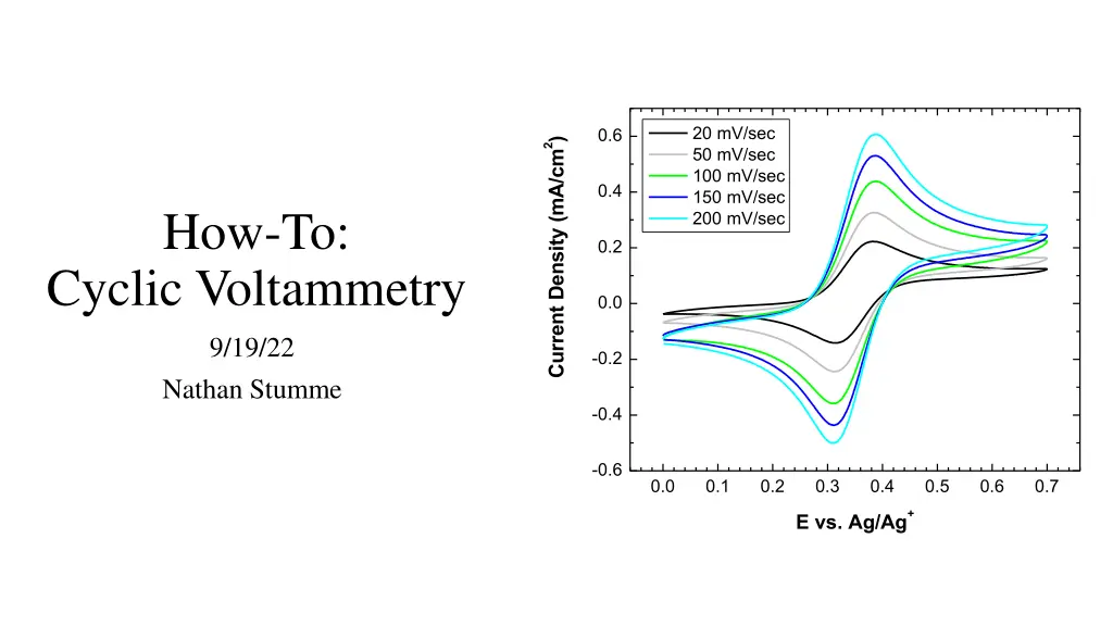
20 mV/sec 50 mV/sec 100 mV/sec 150 mV/sec 200 mV/sec 0.6 2) Current Density (mA/cm 0.4 How-To: 0.2 Cyclic Voltammetry 0.0 9/19/22 -0.2 Nathan Stumme -0.4 -0.6 0.0 0.1 0.2 0.3 0.4 0.5 0.6 0.7 + E vs. Ag/Ag

How-To overview Electrochemical cell, function of electrodes, CV theory, impact of scan rate, embedded chemical steps Common quantitative & qualitative interpretation techniques Practical use: performing CV in the Shaw group 1 2 3 1

The electrochemical cell and electrodes Cyclic voltammetry is an electrochemical technique that measures current (A) as a function of an applied potential (V). It provides both qualitative and quantitative information on the redox processes of species. Electrolyte: the electrolyte is an inert conductive substance dissolved in solution that increases the conductivity and allows electrons to move between the electrodes and solution.(some salt) Working electrode (WE): the potential is directly changed at the WE, and current is measured as electrons move between solution and the WE. Counter electrode (CE): connected in circuit to the WE and passes equal & opposite current to compensate the charge being passed at the WE. You want a CE with a surface area >> WE so the CE can always keep up with the charge being passed at the WE and not limit it. Electrochemistry units Electric charge (e) Faraday s constant (F) Current (A) Coulomb (C) Potential (V) 1 electron = 1.6x10-19 C F = 96485 C/mol electrons A = C/sec C = A*sec V = J/C Reference electrode (RE): connected in circuit to the WE and provides a constant potential for the WE to reference. This is most typically a well- defined and stable redox couple (some version of Ag/Ag+). Modes of mass transport: Quasi-reference electrode (QRE): functions the same as a normal RE but is instead referenced to a well-defined standard redox-active species (ferrocene or cobaltocene) spiked into solution at the conclusion of the experiment. The QRE is usually a Ag or Pt wire. Diffusion: Movement of species due to a concentration gradient. Migration: Movement of species due to a potential gradient (undesirable for CV and mitigated through sufficient electrolyte). Convection: Movement of species due to external force (stirring, pumping, etc.) 2

CV Theory G = -nFE 20 - 2) Current Density (mA/cm 15 A A+ + e- E L E C T R O D E 10 5 HOMO of molecule A E Start E 0 -5 A+ + e- A -10 + 0.0 0.2 0.4 0.6 0.8 1.0 + E vs. Ag/Ag 3

CV Theory G = -nFE 20 - 2) Current Density (mA/cm 15 A A+ + e- E L E C T R O D E Increase in current as A begins diffusing to electrode to undergo oxidation 10 5 HOMO of molecule A E Start E 0 -5 A+ + e- A -10 + 0.0 0.2 0.4 0.6 0.8 1.0 + E vs. Ag/Ag 3

CV Theory G = -nFE 20 - 2) Current Density (mA/cm 15 A A+ + e- E L E C T R O D E Steady current increase as A diffuses to electrode and is oxidized 10 5 HOMO of molecule A E Start E 0 -5 A+ + e- A -10 + 0.0 0.2 0.4 0.6 0.8 1.0 + E vs. Ag/Ag 3

CV Theory G = -nFE 20 - Peak current 2) Peak current is reached as there is depletion of surface [A] and max mass transfer rate is reached. A begins to diffuse in from the bulk solution now. Current Density (mA/cm 15 A A+ + e- E L E C T R O D E 10 5 LUMO of molecule A+ E Start E 0 -5 A+ + e- A -10 + 0.0 0.2 0.4 0.6 0.8 1.0 + E vs. Ag/Ag 3

CV Theory G = -nFE 20 - Peak current 2) Current Density (mA/cm 15 A A+ + e- E L E C T R O D E Decline in current as depletion of surface [A] sets in and the surface [A+] increases 10 5 LUMO of molecule A+ E Start E 0 -5 A+ + e- A -10 + 0.0 0.2 0.4 0.6 0.8 1.0 + E vs. Ag/Ag 3

CV Theory G = -nFE 20 - Peak current 2) Current Density (mA/cm 15 A A+ + e- E L E C T R O D E 10 5 LUMO of molecule A+ E Start E 0 Surface becomes saturated with A+ and mass transport of A from the bulk reaches equilibrium -5 A+ + e- A -10 + 0.0 0.2 0.4 0.6 0.8 1.0 + E vs. Ag/Ag 3

CV Theory G = -nFE 20 - Peak current 2) Current Density (mA/cm 15 A A+ + e- E L E C T R O D E 10 5 LUMO of molecule A+ E Start E Switching potential, scanning in negative direction now 0 -5 A+ + e- A -10 + 0.0 0.2 0.4 0.6 0.8 1.0 + E vs. Ag/Ag 3

CV Theory G = -nFE 20 - Peak current 2) Current Density (mA/cm 15 A A+ + e- E L E C T R O D E 10 5 LUMO of molecule A+ E Start E Increase in current as A+ begins diffusing to electrode to undergo reduction 0 -5 A+ + e- A -10 + 0.0 0.2 0.4 0.6 0.8 1.0 + E vs. Ag/Ag 3

CV Theory G = -nFE 20 - Peak current 2) Current Density (mA/cm 15 A A+ + e- E L E C T R O D E 10 5 LUMO of molecule A+ E Start E Steady current increase as A+ diffuses to electrode and is reduced 0 -5 A+ + e- A -10 + 0.0 0.2 0.4 0.6 0.8 1.0 + E vs. Ag/Ag 3

CV Theory G = -nFE 20 - Peak current 2) Current Density (mA/cm 15 A A+ + e- E L E C T R O D E 10 5 LUMO of molecule A+ E Start E Peak current is reached as there is depletion of surface [A+] and max mass transfer rate is reached. A+ begins to diffuse in from the bulk solution now. 0 -5 A+ + e- A -10 Peak current + 0.0 0.2 0.4 0.6 0.8 1.0 + E vs. Ag/Ag 3

CV Theory G = -nFE 20 - Peak current 2) Current Density (mA/cm 15 A A+ + e- E L E C T R O D E 10 5 LUMO of molecule A+ E Start E 0 Decline in current as depletion of surface [A+] sets in and the surface [A] increases -5 A+ + e- A -10 Peak current + 0.0 0.2 0.4 0.6 0.8 1.0 + E vs. Ag/Ag 3

CV Theory G = -nFE 20 - Peak current 2) Current Density (mA/cm 15 A A+ + e- E L E C T R O D E 10 5 LUMO of molecule A+ E Start E 0 Surface becomes saturated with A and mass transport of A+ from the bulk reaches equilibrium -5 A+ + e- A -10 Peak current + 0.0 0.2 0.4 0.6 0.8 1.0 + E vs. Ag/Ag 3

CV Theory G = -nFE 20 - Peak current 2) Current Density (mA/cm 15 A A+ + e- E L E C T R O D E 10 5 LUMO of molecule A+ E Start E 0 Switching potential, back where we started -5 Disclaimer: the energy of electrode and orbitals of molecules comes in the form of a band, so electrons move in the whole region of the orbital. A+ + e- A -10 Peak current + 0.0 0.2 0.4 0.6 0.8 1.0 + E vs. Ag/Ag 3

Important spots in the CV 20 G = -nFE Go = -nFEo Oxidation peak current & E G = Go + RTln(Q) 2) Current Density (mA/cm 15 E1/2 10 -nFE = -nFEo + RTln(Q) divide by -nF 5 E = Eo - (RT/nF)ln(Q) Nernst equation Switching E Start E 0 The E1/2 value is called the formal potential and is where the surface concentration of each species (A and A+) are equal. In the Nernst equation, this cancels out the second term, and E = Eo. This is what is reported for a redox couple. -5 -10 Reduction peak current & E 0.0 0.2 0.4 0.6 0.8 1.0 + E vs. Ag/Ag 4

Changing the scan rate changes your CV As the potential is changed at different rates, the amount of current passed at the oxidation and reduction peak currents changes. This phenomenon can be rationalized by looking at the units of current (A = C/s). 20 mV/sec 50 mV/sec 100 mV/sec 150 mV/sec 200 mV/sec 0.6 2) Current Density (mA/cm 0.4 0.2 When applying faster scan rates, there is less time to pass the same number of coulombs (C) at the electrode surface (surface area dependent). Because of this, larger peak currents are observed as there is a smaller time value in the denominator. 0.0 -0.2 -0.4 Varying the applied scan rate is useful for both qualitatively and quantitatively interpreting your CVs. -0.6 0.0 0.1 0.2 0.3 0.4 0.5 0.6 0.7 + E vs. Ag/Ag 5

CVs can have multiple redox features 3 2) Current Density (mA/cm 2 1 Example: each of the nitrogen atoms on this molecule can undergo reversible oxidations. This leads to two reversible redox features in the CV. 0 -1 Mechanism: A A+ + e- A+ A2+ + e- A2+ + e- A+ A+ + e- A -2 -0.2 0.0 0.2 0.4 0.6 0.8 1.0 1.2 1.4 + E vs. Fc/Fc 6

It isnt always so clean reversibility & chemical steps Reversible peak splitting math E = Eo - (RT/nF)ln(Q) Nernst equation 8.314 ? 298 ? ??? 96485 ? ??? ? = 0.05916? ?= 0.05916 ? Chemical steps A chemical step involves a chemical reaction coupled to the electron transfer. In this example, the mechanism looks something like: A A+ + e- A+ + B C A+ + e- A (doesn t occur) Reversible: redox feature with equal oxidation/reduction peak currents (areas) with peak splitting ~60-80 mV (59 mV peak splitting is the ideal value for a 1 electron transfer due to the Nernst equation RT/nF = 0.05916 V difference for a redox couple.) ~29.5 mV splitting for 2 e- transfer. Quasi-reversible: redox feature with ~equal oxidation/reduction peak currents (areas) with peak splitting 80-250 mV. Indicates slower electron transfer kinetics. This is called an EC mechanism (electron transfer, chemical reaction) Irreversible: redox feature with unequal oxidation/reduction peak currents and/or peak splitting > 250 mV. Indicates very slow electron transfer kinetics and possibly chemical steps. 7

Another chemical step mechanism example Types of steps: E = electron transfer (rev or irrev) C = chemical reaction (rev or irrev) C* = catalytic step, generates product and regenerates reactant An important note: You can often tease out chemical steps and mechanisms by varying the scan rate. At slow scan rates the chemical reaction may have time to occur, but at faster scan rates you may outrace the chemical reaction and catch the electron transfer. Doing this is super helpful for understanding your system. ECE mechanism A A+ + e- A++ B C C C+ + e- C+ + e- C A+ + e- A (doesn t occur) 8

One silly thing- different CV conventions There are unfortunately two different conventions for reporting CV data, the US (Texas) and IUPAC conventions. They are just rotated by 180o and have oxidation/reduction and high/low potentials flipped flopped. You will see both variants in literature, but for all cases moving to positive potentials = oxidation and moving to negative potentials = reduction. 9

Quantitative data from CV data diffusion coefficient Diffusion Coefficient (cm2/sec) D: The diffusion coefficient tells you how quickly a species diffuses to the electrode to undergo electron transfer. This is typically calculated using theRandles ev k equation, which connects the peak current in A to the square root of the applied scan rate in V to calculate D for a diffusion-controlled electrochemical process. D is usually calculated by obtaining CVs at varying scan rates (~5) and plotting the oxidation and reduction peak currents for each vs. the square root of the applied scan rate (D is calculated for oxidation and reduction respectively). The slope of this line is ip/v1.5 for all data points and should be a straight line (R2 = 0.99+). By plugging in other known variables, you can solve for D. Alternatively, if you know D for a species, you can use it to solve for the concentration of the solution, as the # of electrons passed scales with the # of mols of species present. You can also solve for the surface area of the electrode. Something to note: If your peak currents are linear with just the scan rate (not the square root), you have an adsorption-controlled process occurring. 10

Quantitative data from CV data heterogeneous electron transfer rate Heterogeneous electron transfer rate (cm/sec) k0: As the name implies, the electron transfer rate tells you the kinetics of an electron transfer. There are unfortunately many ways to go about doing this depending on the situation, but the most common and user-friendly is the Nicholson method. All methods rely in some way on the difference in potential ( E) between oxidation and reduction peak currents and the diffusion coefficient. Like D, k0 also requires obtaining CVs at varying scan rates. For the Nicholson method, the two above equations are needed. Psi is a dimensionless value developed by Nicholson that accounts for the reversibility of the electron transfer (peak splitting). X is the peak splitting ( E) in mV for your redox feature. Psi can be determined for each scan rate in [3] by inserting the peak splitting values (X). These Psi values are then plotted against the entire right side of [2] except for k0 for each scan rate. The slope of this line provides k0. 11

Practical CV in the Shaw group Main skills: Choosing your electrodes, electrolyte, and solvent Electrode preparation (mechanical polishing and flame polishing) Using the potentiostat software (CHI) Data saving Data workup 12

Choosing your electrodes, electrolyte, & solvent 0.6 2) 0.4 Full solvent window Current Density (mA/cm 0.2 0.0 -0.2 -0.4 -0.6 -0.8 -4 -3 -2 -1 0 1 + E vs. Fc/Fc Disc WE options we have: glassy carbon, platinum, gold, silver (some others too but these are the main ones you d use) When choosing your WE, CE, and RE, electrolyte, and solvent you want to ensure you are using a combination that is electrochemically inert in the potential window you are studying. Obtaining a background window with electrodes and electrolyte is good practice. 13

Electrode preparation: mechanical polishing To mechanically polish disc working electrodes, you will use Buehler microcloth PSA pads with an aqueous slurry of alumina powder (1.0 micron followed by 0.3 micron size). Make a slurry on the pad, and gently press the working electrode straight onto the pad and move it in a figure eight motion for roughly 60-90 seconds. After this, rinse it off using ultrapure water and sonicate for ~5 minutes in a vial (shown right). After sonication, repeat with the smaller micron size pad. Disclaimer: Do NOT sonicate the glassy carbon working electrode, it has epoxy holding the glassy carbon to the electrode, which is worn down with sonication and destroys the electrode over time. 14

Electrode preparation: flame polishing To flame polish metal wire electrodes, you will use the hydrogen torch in the instrument lab. The hydrogen valve is red and turning it to the left opens it. Leave the valve shut and pressurize the hydrogen tank first, making sure the regulator isn t pressurized when opening the main tank valve. Pressurize the regulator to ~5 psi (first line) and open the red valve on the torch in the hood. You shouldn t hear hydrogen hissing loudly, it only needs to be opened a little. Light the hydrogen with the sparker in the hood and adjust so the flame is 2-3 inches high and isn t making any noise. Put your metal wire in the hydrogen flame until it glows red and then pull it out. Do this several times, being careful to not get too close to the soldered connection as the flame can melt your solder. Once finished, close the red valve and then close the main valve on the hydrogen tank to stop the supply of hydrogen. Reopen the red valve to vent all hydrogen from the regulator and then loosen the regulator so it doesn t accidentally automatically pressurize for the next person. (Don t flame polish the disc working electrodes) 15

Potentiostat and wire connections To acquire a CV, make sure the potentiostat is plugged into the wall and turn it on using the on button located on the back of the potentiostat. Make sure the potentiostat is connected to the computer with the USB plug too. Connect the leads coming from the potentiostat to your electrodes in your electrochemical cell. For CHI, green = WE, red = CE, and white = RE. Make sure the wires are freely hanging and aren t being pulled taught or bent in a weird way. 16

Potentiostat software This is the window when you open the CHI software, the main buttons you will use are shown in arrows. 17

Potentiostat software Clicking on the T, you can choose which technique you want to use (cyclic voltammetry). 18

Potentiostat software Clicking on the checklist, you can then change your relevant CV parameters. You can choose your initial V, high V, low V, and final V, and the scan polarity tells you which way you ll scan first. You can also change the scan rate, the number of sweep segments (times back and forth), number of data points (sample interval), time until it starts taking the CV (quiet time) and sensitivity (how much current you can pass). When you are ready, click the run button to acquire the CV. You should always do at least 4 segments and ignore the first full sweep, because gunk on the electrode leads to varying currents and inaccurate data on your first cycle. The CV settles in after the first sweep for all the subsequent ones. 19

Data saving To save data, click file Save as and choose the location you want to save. You can save files as .bin files and .csv files. The .bin files are the proprietary file for CHI which you can only open in their software, and the .csv files are Excel readouts of E and current. I recommend saving in both file types. You can also save as a .txt file if that is more convenient (same readout as the .csv). 20

Data workup With your raw data, you will have column readouts of potential (V) and current (A). Copy one of your middle/final cycles to use as your data set. You will typically want to plot your data as current density (mA/cm2) vs. E (vs. some RE). To normalize for current density, divide your current values by the surface area of your working electrode (geometric or preferably electrochemically determined from a Randles ev k study with potassium ferricyanide). If you have used a Ag/Ag+ variant RE, your potentials are already correct. If using a QRE to Fc/Fc+ you will need to subtract the E1/2 value of the Fc/Fc+ redox couple that you spiked into your solution from each E value. This will make your E axis relative to the Fc/Fc+ redox couple. Plot in Origin and you re set. D and k0 can be calculated from your data set using Excel. 3 2) Current Density (mA/cm 2 1 0 -1 -2 -0.2 0.0 0.2 0.4 0.6 0.8 1.0 1.2 1.4 + E vs. Fc/Fc 21

Helpful resource I would highly recommend reading this journal article (even if CV isn t your thing), it is without a doubt the most concise and useful article I have encountered in graduate school, and I refer back to it often. It s only about a 15-minute read in total and it covers all the essentials for cyclic voltammetry. (As you can tell it s a popular one) https://pubs.acs.org/doi/10.1021/acs.jchemed.7b00361 22