Understanding Eigenvalues of Ordinary Differential Equations and Finite Difference Techniques
Explore the concepts of eigenvalues of ordinary differential equations and finite difference techniques through a simple model problem, matrix equations, and MATLAB code. Learn how to choose a mesh, solve for eigenvalues, and analyze results for different values of n.

Uploaded on | 1 Views
Download Presentation

Please find below an Image/Link to download the presentation.
The content on the website is provided AS IS for your information and personal use only. It may not be sold, licensed, or shared on other websites without obtaining consent from the author. If you encounter any issues during the download, it is possible that the publisher has removed the file from their server.
You are allowed to download the files provided on this website for personal or commercial use, subject to the condition that they are used lawfully. All files are the property of their respective owners.
The content on the website is provided AS IS for your information and personal use only. It may not be sold, licensed, or shared on other websites without obtaining consent from the author.
E N D
Presentation Transcript
Eigenvalues of Ordinary Differential Equations Jake Blanchard University of Wisconsin
Introduction Finite Difference Techniques Matlab
Model Problem A simple eigenvalue problem 2 d y dx + = 2 y 0 2 = = y ( ) 0 y ( ) 1 0 Solution = n , n = n x sin( ) y A n n
Finite Difference Solution + y 2 y 2 y + + = 2 i 1 i i 1 y 0 i h + = 2 2 y ( 2 h ) y y 0 + i 1 i i 1
Choosing a Mesh Divide range 0<x<1 into 8 regions This produces 9 mesh points Boundary conditions eliminate two unknowns We re left with 7 unknowns (the 7 internal mesh points)
Matrix Equation 1 0 0 0 0 0 2 1 0 1 0 0 1 0 0 0 1 0 0 0 0 1 0 0 0 0 0 1 1 0 0 0 0 2 1 0 0 0 2 y 1 0 0 + = 2 2 2 y h 0 1 0 2 1 2 2 i 2= 2 h e i
Code n=7; h=1/(n+1); voffdiag=ones(n-1,1); mymat=-2*eye(n)+diag(voffdiag,1)+diag(voffdiag,-1); D=sort(eig(mymat),'descend'); lam=sqrt(-D)/h; check=lam/pi; myint=(1:n)'; plot(myint,check,myint,myint) myerr=abs(check-myint)./(myint); figure semilogy(myint,myerr)
Results n=7 7 6 5 4 3 2 1 0 1 2 3 4 5 6 7
Results (error) n=7 0 10 -1 10 -2 10 -3 10 1 2 3 4 5 6 7
Results n=2000 2000 1800 1600 1400 1200 1000 800 600 400 200 0 0 200 400 600 800 1000 1200 1400 1600 1800 2000
Results (error) n=2000 0 10 -1 10 -2 10 -3 10 -4 10 -5 10 -6 10 -7 10 0 200 400 600 800 1000 1200 1400 1600 1800 2000


 – n=7")

 – n=2000")