Understanding Experimental Designs and T-Tests in Research

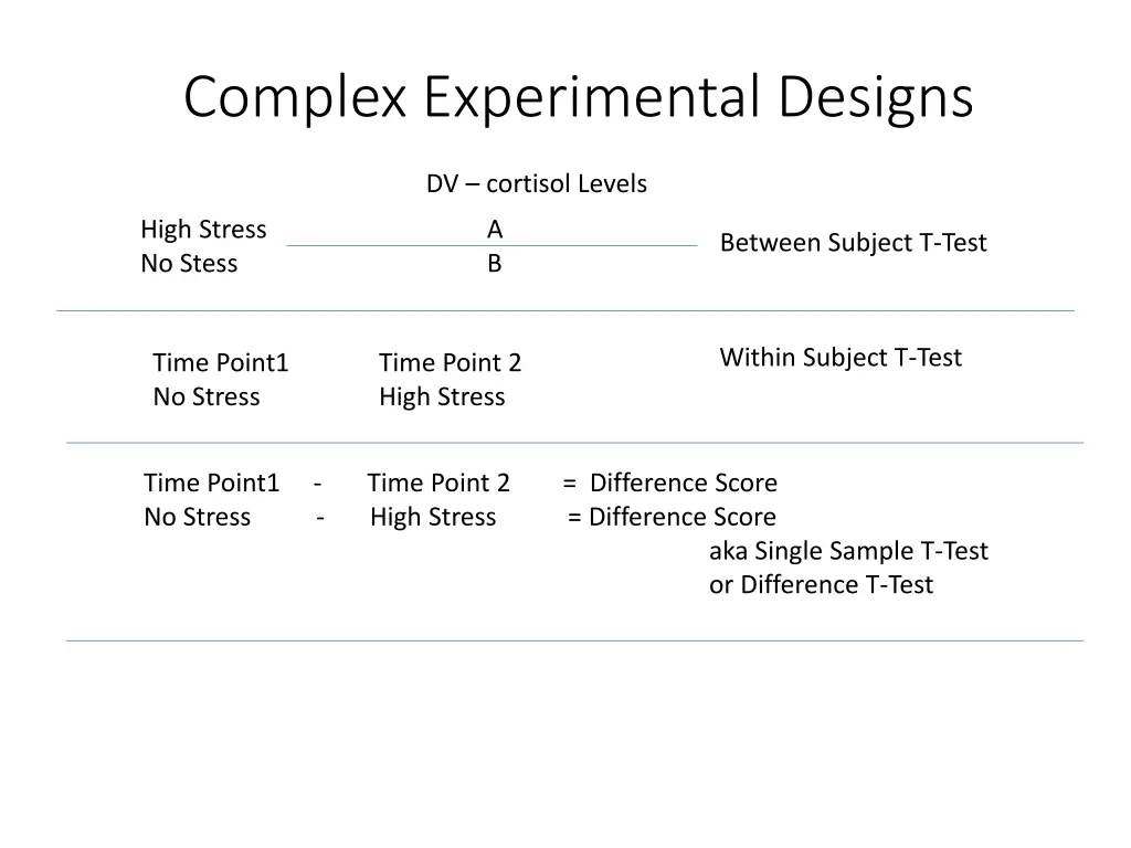
Complex Experimental Designs DV cortisol Levels High Stress No Stess A B Between Subject T-Test Within Subject T-Test Time Point1 No Stress High Stress Time Point 2 Time Point1 - Time Point 2 = Difference Score No Stress - High Stress = Difference Score aka Single Sample T-Test or Difference T-Test

Assumptions of a T-Test 1. DV is continuous 2. Your independent variable should consist of two categorical, independent groups. 3. You should have independence of observations, which means that there is no relationship between the observations in each group or between the groups themselves. 4. There should be no significant outliers. 5. Your dependent variable should be approximately normally distributed for each group of the independent variable. 6. There needs to be homogeneity of variances. 2

Increasing the number of levels of the independent variables The simplest experimental design has an IV with only 2 levels However, it is often desirable to include more than 2 levels of the IV E.g., When you expect to find a curvilinear relationship or when you need more fine-grained information How far can you go? How far should you go? Depends on the relationship between the IV and DV? Depends on how many subjects you want to get? Depends on if you want to look at an interaction? 3

Increasing the number of levels of the independent variables E.g., Testing the Yerkes-Dodson law 4

Increasing the number of independent variables The simplest experimental design has only one IV E.g., Consuming beer and fake beer before driving on a simulator However, it is possible (and, in fact, more common) to have more than one IV in an experiment = Factorial design DV1 DV2 DV3 High Stress Medium Stress Low Stress Anti-Anxiety Drug A High Stress Medium Stress Low Stress Anti-Anxiety Drug B 2x3x3 5

2x2 TV Violence and Supervision TV violence Low High Present Supervision Absent 6

Factorial design Question: How many IVs are there in a 3 x 3 Factorial Design? Answer: 2 2 x 2 x 2 2x 3 x 3 2 x 2 x 2 x 2 Repeat the above if this was a Mixed Factorial Design 7

DVT1 DVT2 DVT3 High Stress Medium Stress Low Stress Anti-Anxiety Drug A High Stress Medium Stress Low Stress Anti-Anxiety Drug B Main Effects Unique effect of a particular variable on a dependent or outcome variable Interactions - Combine effect of two or more IV or predictor variables on a DV or outcome variable 8

Interpretation of factorial design TV violence Low High 1.5 4.5 3.0 Present Supervision 2.5 8.5 5.5 Absent 2.0 6.5 4.25 9

Interpretation of factorial design 10 9 8 7 Supervision 6 No supervision 5 4 3 2 1 Low violence High violence 10

Interpretation of factorial design 10 9 8 7 6 Supervision 5 No supervision 4 3 2 1 Low violence High violence 11

12

13

14

The search for moderators 15

More Practice 16

Terminology Main effect Interaction Moderator variable Simple main effect (of each IV at a particular level of another IV) Mixed factorial design Between & within subjects 17

Independence of cases this is an assumption of the model that simplifies the statistical analysis. Normality the distributions of the residuals are normal. Equality (or "homogeneity") of variances, called homoscedasticity... Point of interest here is the second assumption. Several sources list the assumption differently. Some say normality of the raw data, some claim of residuals. Several questions pop up: are normality and normal distribution of residuals the same person (I would claim normality is a property, and does not pertain residuals directly but can be a property of residuals? if not, which assumption should hold? One? Both? if the assumption of normally distributed residuals is the right one, are we making a grave mistake by checking only the histogram of raw values for normality? 18

Mixed Designs: Between and Within

Complex Designs Multiple IVs Multiple DVs Why? 20

The mixed factorial design is, in fact, a combination of these two. It is a factorial design that includes both between and within subjects variables. One special type of mixed design, that is particularly common and powerful, is the pre-post-control design. This is a design in which all subjects are given a pre- test and a post-test, and these two together serve as a within-subjects factor (test). Participants are also divided into two groups. One group is the focus of the experiment (i.e., experimental group) and one group is a base line (i.e., control) group. So, for example, if we are interested in examining the effects of a new type of cognitive therapy on depression, we would give a depression pre-test to a group of persons diagnosed as clinically depressed and randomly assign them into two groups (traditional and cognitive therapy). After the patients were treated according to their assigned condition for some period of time, let s say a month, they would be given a measure of depression again (post-test). This design would consist of one within subject variable (test), with two levels (pre and post), and one between subjects variable (therapy), with two levels (traditional and cognitive) (Figure 1). Pre-Test Cognitive Pre Traditional Pre Post-Test Cognitive Post Traditional Post Cognitive Therapy Traditional Therapy 2x2 21

When a researchers uses the pre-post-control design he or she is usually looking for an interaction such that one cell in particular stands out, and that is the experimental group s post test score. Ideally the pre-test scores will be equivalent. It is the post-test score difference between the experimental and control group that is important (see Figure 2). Figure 2. Hypothetical Means for Experiment in Figure 1 22

Therefore, in terms of post-hoc tests the most important comparison is between the post-test mean for the experimental group and the post-test mean for the control group (see Figure 3). Figure 3. Comparison of Post-Test Means Also, it is typical for the experimenter to expect a change in the experimental group from pre to post, but not in the control group, which would make the important post-hoc comparisons between pre- and post-test for the experimental groups and between pre- and post-test for the control group (see Figure 4). Post hoc ergo propter hoc

Figure 4. Comparison of Pre vs. Post Test Means for Both Groups Of course, the pre-post-control design is not the only type of mixed design. Another common type of mixed design (and within-subjects design in general) is one that includes a change over time, so that one independent variable consists of multiple measures of one group of people over time. So, for example, we might be interested in comparing the interest of males vs. females in math and science over some time period during development. More specifically, we could give a group of school children a measure of interest in math and science at age 10 and then give the same group of students the same measure of interest at age 18. Our design then would look like Figure 5, and one set of possible means would look like the means in Figure 6, which would represent an interaction. Figure 5. Mixed Design with Time as a Within-Subjects Factor Figure 6. Hypothetical Means for the Experiment in Figure 5 Age 10 Age 18 Males Males-Age 10 Males-Age 18 Females Females- Age 10 Females- Age 18 24

Figure 7. Flow Chart Representing Choice of Analysis Depending on Design 25

Mixed Between and Within Designs Conceptualizing the Design Types of Mixed Designs Assumptions Analysis Deviation Computation Higher order mixed designs Breaking down significant effects

Conceptualizing the Design This is a very popular design because you are combining the benefits of each design Requires that you have one between groups IV and one within subjects IV Often called Split-plot designs, which comes from agriculture In the simplest 2 x 2 design you would have

Conceptualizing the Design In the simplest 2 x 2 design you would have subjects randomly assigned to one of two groups, but each group would experience 2 conditions (measurements) GRE - before GRE - after S1 S2 S3 S4 S5 S6 S7 S8 S9 S10 S1 S2 S3 S4 S5 S6 S7 S8 S9 S10 Kaplan Princeton

Conceptualizing the Design Advantages First, it allows generalization of the repeated measures over the randomized groups levels Second, reduced error (although not as reduced as purely WS) due to the use of repeated measures Disadvantages The addition of each of their respective complexities

Conceptualizing the Design Types of Mixed Designs Other than the mixture of any number of BG IVs and any number of WS IVs Pretest Posttest Mixed Design to control for testing effects Pretest S1 S2 S3 S4 S5 S6 S7 S8 S9 S10 Posttest S1 S2 S3 S4 S5 S6 S7 S8 S9 S10 Treatment Group Treatment Control Group No Treatment

Assumptions Normality of Sampling Distribution of the BG IVs Applies to the case averages (averaged over the WS levels) Homogeneity of Variance Applies to every level or combination of levels of the BG IV(s)

Assumptions Independence, Additivity, Sphericity Independence applies to the BG error term and means .. An assumption that one data point does not influence another behavior of one does not influence the other But each WS error term confounds random variability with the subjects by effects interaction so we need to test for sphericity instead; the test is on the average variance/covariance matrix (over the levels of the BG IVs) can be defined as . Variances of differences between data taken form the same participants are equal Additivity

Assumptions Outliers Look for them in each cell of the design Missing data Causes the same problems that they did in the BG and WS designs separately Data points missing across the WS part can be estimated as discussed previously Missing data in the randomized groups part causes non-orthogonality

Analysis Within Groups b1 S1 S2 S3 S4 S5 S6 S7 S8 S9 S10 S11 S12 S13 S14 S15 b2 S1 S2 S3 S4 S5 S6 S7 S8 S9 S10 S11 S12 S13 S14 S15 b3 S1 S2 S3 S4 S5 S6 S7 S8 S9 S10 S11 S12 S13 S14 S15 a1 Randomized Groups a2 a3

Sources of Variance SST=SSBG+SSWS What are the sources of variance? A S/A B AB BxS/A T Degrees of freedom?

Example Books by Month Example: Imagine if we designed the previous research study concerning reading different novels over time But instead of having everyone read all of the books for three months we randomly assign subjects to three different books and have them read for three months

B: Month b1: b2: b3: Month 1 1 Month 2 3 Month 3 6 Case Means S1 S2 S3 S4 S5 S1 = 3.333 S2 = 4.333 S3 = 4 S4 = 5.667 S5 = 3.667 a1 = 4.2 S6 = 1.333 S7 = 3.333 S8 = 3.333 S9 = 2 S10 = 4 a2 = 2.8 S11 = 2 S12 = 3 S13 = 3 S14 = 3 S15 = 2.667 a3 = 2.733 1 4 8 a1: Science Fiction 3 3 6 5 5 7 2 4 5 a1b1 = 2.4 a1b2 = 3.8 a1b3 = 6.4 3 1 S6 S7 S8 S9 S10 a2 0 A: Type of Novel 4 4 2 a2: Mystery 5 3 2 4 2 0 4 5 3 a2b1 = 4 4 a2b2 = 3 2 a2b3 = 1.4 0 S11 S12 S13 S14 S15 2 6 1 a3: Romance 3 3 3 6 2 1 3 3 2 a3b1 = 3.6 a3b2 = 3.2 a3b3 = 1.4 b1 = 3.333 b2 = 3.333 b3 = 3.067 GM = 3.244

Sums of Squares - Deviation The total variability can be partitioned into A, B, AB, S/A, and B*S/A = + + + + SS SS SS SS SS SS / * / B S A Total A B AB S A ( ) ( ) ( ) 2 2 2 = + + Y Y n Y Y n Y Y ... . . j ... .. ... ijk j k k ( ) ( ) ( ) 2 2 2 + n Y Y n Y Y n Y Y . ... . . j ... .. ... jk jk j k k ( ) ( ) ( ) 2 2 2 + + j Y Y Y Y j Y Y .. . . j . .. . . k i ijk jk i

( ) 2 ( ) ( ) ( ) 2 2 2 = = + 2.8 3.244 + 2.733 3.244 ] 20.583 = 15*[ 4.2 3.244 SS n Y Y . . j ... A j ( ) ( ) ( ) ( ) 2 2 2 2 = = + 3.333 3.244 + 3.067 3.244 ] .708 = 15*[ 3.333 3.244 SS n Y Y .. ... B k k ( ) ) ( ) ( ) 2 2 2 = = SS n Y Y n Y Y n Y Y . ... . . j ... .. ... AB jk jk j k k ( + 2 ( ) ( ) ( ) 2 2 2 = *[ 2.4 3.244 + 3.8 3.244 + 6.4 3.244 + 5 n Y Y . ... jk jk ( ( ) ( ) ( ) = ) 2 2 2 4 3.244 + 3 3.244 + 1.4 3.244 + ) ( ( ) 2 2 2 + 3.6 3.244 = + 3.2 3.244 + 1.4 3.244 ] 92.711 = 92.711 20.583 .708 71.420 SS AB

( ) 2 ( ) ( ) ( ) 2 2 2 = = + + 4 4.2 + 3*[ 3.333 4.2 4.333 4.2 SS k Y Y / .. . . j S A i ( ( ( ) ) ( ( ) ( ) ( ) ( ) 2 2 2 2 2 + + + + + + 5.667 4.2 3.667 4.2 3.333 2.8 1.333 2.8 3.333 2.8 ) ( ) ( ) ( ) 2 2 2 2 2 + + 2 2.8 + 2 2.733 + 3 2.733 + 3 2.733 + 3.333 2.8 ) ( ) 2 2 + 3 2.733 + 2.667 2.733 ] = 26.400

( ) ( ) 2 2 = = SS Y Y k Y Y * / B S A . .. . . j ijk jk i ( ) 2 ( ) ( ) ( ) ( ) ( ) 2 2 2 2 2 = 1 2.4 + 1 2.4 + 3 2.4 + 5 2.4 + 2 2.4 + Y Y . ijk jk ( ( ( ( ( ( ( ( ) ) ( ( ) ) ( ( ) ) ( ( ) ( ) 2 2 2 2 2 + 3 3.8 + 4 3.8 + 3 3.8 + 5 3.8 + 4 3.8 + ) ( ) 2 2 2 2 2 + 6 6.4 + 8 6.4 + 6 6.4 + 7 6.4 + 5 6.4 + ) ( ) ( ) ( ) ( ) 2 2 2 2 2 + 3 4 + 4 4 + 5 4 + 4 4 + 4 4 + ) ( ) ( ) ) ) ) ) ( ) ( ( ) 2 2 2 2 2 + 1 3 + ) ) ) ) 4 3 ( ( ( ( 1 1.4 63.6 26.4 + 3 3 + 2 3 + 5 3 + ( ) ) ( ) 2 2 2 2 2 + 0 1.4 + 2 1.4 + 2 1.4 + 0 1.4 + 3 1.4 + ( ( ) ) ( ( ) ) ( ( ) ) 2 2 2 2 2 + 4 3.6 + 2 3.6 + 3 3.6 + 6 3.6 + 3 3.6 + 2 2 2 2 2 + 2 3.2 + 6 3.2 + 3 3.2 + 2 3.2 + 3 3.2 + ( ) ( ) ( ) 2 2 2 2 2 + 0 1.4 + + + 1 1.4 + 2 1.4 = 3 1.4 37.2 63.6 = = SS * / B S A

( ) 2 = = SS Y Y ... Total ijk ( ) ( ) ( ) ( ) ( ) 2 2 2 2 2 = 1 3.244 + 1 3.244 + 3 3.244 + 5 3.244 + 2 3.244 + SS Total ( ( ( ( ( ( ( ( ) ) ) ) ) ) ) ) ( ( ( ( ( ( ( ( ) ) ) ) ) ) ) ) ( ( ( ( ( ( ( ( ) ) ) ) ) ) ) ) ( ( ( ( ( ( ( ( ) ) ) ) ) ) ) ) ( ( ( ( ( ( ( ( ) ) ) ) ) ) ) ) 2 2 2 2 2 + 3 3.244 + 4 3.244 + 3 3.244 + 5 3.244 + 4 3.244 + 2 2 2 2 2 + 6 3.244 + 8 3.244 + 6 3.244 + 7 3.244 + 5 3.244 + 2 2 2 2 2 + 3 3.244 + 4 3.244 + 5 3.244 + 4 3.244 + 4 3.244 + 2 2 2 2 2 + 1 3.244 + 4 3.244 + 3 3.244 + 2 3.244 + 5 3.244 + 2 2 2 2 2 + 0 3.244 + 2 3.244 + 2 3.244 + 0 3.244 + 3 3.244 + 2 2 2 2 2 + 4 3.244 + 2 3.244 + 3 3.244 + 6 3.244 + 3 3.244 + 2 2 2 2 2 + 2 3.244 + 6 3.244 + 3 3.244 + 2 3.244 + 3 3.244 + 2 2 2 2 2 + 0 3. + 1 3.244 + 3 3.244 + 1 3.244 + 2 3.244 = 244 156.311

B: Month b1: b2: b3: Month 1 1 Month 2 3 Month 3 6 Case Total S1 S2 S3 S4 S5 S1 = 10 S2 = 13 S3 = 12 S4 = 17 S5 = 11 a1 = 63 S6 = 4 S7 = 10 S8 = 10 S9 = 6 S10 = 12 a2 = 42 S11 = 6 S12 = 9 S13 = 9 S14 = 9 S15 = 8 a3 = 41 Total = 146 1 4 8 a1: Science Fiction 3 3 6 5 5 7 2 4 5 a1b1 = 12 a1b2 = 19 a1b3 = 32 3 1 S6 S7 S8 S9 S10 0 4 4 2 A: Type of Novel a2: Mystery 5 3 2 4 2 0 4 5 3 a2b1 = 20 a2b2 = 15 4 a2b3 = 7 0 S11 S12 S13 S14 S15 2 2 6 1 a3: Romance 3 3 3 6 2 1 3 3 2 a3b1 = 18 a3b2 = 16 b1 = 50 a3b3 = 7 b3 = 46 b2 = 50

Sums of Squares - Computational What are the degrees of freedom? And convert them into the formulas A = a - 1 S/A = a(s 1) = as - a B = b - 1 AB = (a 1)(b 1) BxS/A = a(b 1)(s 1) T = abs 1 or N - 1

= = = = = = = 1 3 1 ( 1) 1 3 1 1)( ( 1 abs = 2 df df df df df df a = A = = 3(5 1) 12 2 1) (3 1)(3 1) 1)( 1) 1 3(3)(5) 1 N = a s / S A b B = = ( = 4 a b AB = 3(3 1)(5 1) = = 24 a b s / BxS A = 44 T

Results ANOVA summary table

Higher order mixed designs

Breaking down significant effects Between Groups IV(s) If you have a significant BG main effect(s) they need to be broken down to find which levels are different The comparisons are done the same way as completely BG comparisons The BG comparison error term is the same for all BG comparisons SS 2 2 j ( ) / n w Y MS w ( . ) reg X j j = = Y F j MS / / S AB S AB