Understanding Finance: Risk and Return in Investment Strategies
Dive into the world of finance with a focus on risk and return in investment strategies. Explore concepts such as Markowitz Portfolio Theory, Efficient Frontier, and the impact of lending and borrowing at the risk-free rate. Learn how combining assets can lead to optimal portfolio construction and risk management.

Download Presentation

Please find below an Image/Link to download the presentation.
The content on the website is provided AS IS for your information and personal use only. It may not be sold, licensed, or shared on other websites without obtaining consent from the author. If you encounter any issues during the download, it is possible that the publisher has removed the file from their server.
You are allowed to download the files provided on this website for personal or commercial use, subject to the condition that they are used lawfully. All files are the property of their respective owners.
The content on the website is provided AS IS for your information and personal use only. It may not be sold, licensed, or shared on other websites without obtaining consent from the author.
E N D
Presentation Transcript
Introduction to Finance Risk & Return Expanded Dr Valeriya Vitkova Faculty of Finance
Markowitz Portfolio Theory Expected Returns and Standard Deviations vary given different weighted combinations of the two stocks Expected Return (%) IBM 40% in IBM Wal-Mart Standard Deviation V Vitkova 2
Efficient Frontier Assume that we have 10 stocks. The grey area in the graph below shows all the possible portfolio combinations between the 10 stocks. The various weighted combinations of stocks on the pink line constitute the set of efficient portfolios. These are portfolios that offer the least risk for a given level of return and the highest return for a given level of risk. Rational investors are only willing to hold efficient portfolios. 3 V Vitkova
Efficient Frontier Here we have expanded the set of possible investments to include all the stocks in the market. Each half egg shell represents possible weighted combinations of different stocks. The efficient frontier is the set of all efficient portfolios. Expected Return (%) Here we are considering all the stocks in the market and we know that stocks are risky assets What happens when we introduce the possibility to invest in the risk-free asset? V Vitkova Standard Deviation 4
Lending and Borrowing at the Risk-free Rate What happens to our set of investment opportunities if we can borrow and lend at the risk-free rate? In finance, the risk-free rate is defined as the rate of return (yield to maturity) offered by short-term government bonds The short-term typically refers to government bonds with time to maturity of less than one year An example of the risk-free rate of return is the return (yield to maturity) of US government Treasury bills We are lending at the risk-free rate if we invest in US Treasury bills (i.e. we buy some Treasury bills) We are borrowing at the risk-free rate if we can get a loan from the bank at the risk-free rate V Vitkova 5
Efficient Frontier with lending and borrowing What happens to the efficient frontier when we introduce the possibility to borrow and lend at the risk-free rate? We now have new portfolios which are combinations between our risky portfolio and the risk-free asset The return on these new portfolios is a weighted average of the return of the risky portfolio and the return of the risk-free asset The risk of these new portfolios is: = + x ( 2 + 2 1 2 1 2 2 2 2 Portfolio Variance x x x ) 1 2 12 1 2 If X2 is the fraction invested in the risk-free asset and ?2 is the risk of the risk-free asset, then ?2= 0, by definition because the risk-free asset has zero risk. The risk of my new portfolio becomes: = 2 1 2 1 New Portfolio Variance x V Vitkova 6
Efficient Frontier with lending and borrowing So how can we find the new efficient frontier graphically? The new efficient frontier is a straight line (the risk is directly proportionate to the level of risk of the risky portfolio, the return is directly proportionate to the returns of the two assets) Let s denote with rf the risk-free asset. Rf plots on the Y axis since it has zero standard deviation We start from the point on the Y axis that is rf and we want to find the best efficient portfolio (lowest risk and highest return). If we draw a straight line from rf , the tangent point to the old efficient frontier (which consists of risky portfolios only) will be the optimal (best) risky portfolio. All investors will want to hold some fraction of this optimal portfolio V Vitkova 7
Efficient Frontier Lending or Borrowing at the risk-free rate (rf) allows us to exist outside the old efficient frontier. It allows all investors to improve their risk and return position. The set of combinations between investing in the risk-free asset and investing in a risky portfolio will be a straight line. Expected Return (%) P This is because the risk- free asset has a standard deviation of zero. K M rf The risk will be measured by ?1?1where ?1is the percentage invested in the risky portfolio (M) and ?1is the standard deviation of the risky portfolio (M). Standard Deviation 8 V Vitkova
Efficient Frontier The red line on the graph below shows all the different possible combinations between portfolio M and the risk-free asset. By changing the percentages invested in the risk-free asset and portfolio M you can achieve any position on the red line. Expected Return (%) If you hold portfolio T, when we introduce borrowing or lending at the risk-free rate, you can improve your position by investing in a combination of portfolio M and the risk-free asset. Portfolio K is an example of this since it offers the same return as portfolio T but for less risk. K M rf T Standard Deviation 9 V Vitkova
Efficient Frontier Similarly, if you hold portfolio G, you can improve your position by investing in a combination of portfolio M and the risk-free asset. Portfolio P is an example of this since it offers the same return as portfolio G but for less risk. Expected Return (%) P G At points between rfand M we are lending at the risk-free rate. At points beyond M we are borrowing at the risk- free rate. M rf Standard Deviation V Vitkova 10
Efficient Frontier The line which is tangent to the efficient frontier shows the optimal risky portfolio (M). Every investor wants to hold combinations between portfolio M and the risk- free asset. It does not make sense to invest in any other portfolio on the efficient frontier when we have a risk-free asset. Expected Return (%) This is because the combinations between the risk-free asset and any other portfolio will be inefficient. For example, look at the green line which shows combinations between portfolio T and the risk free asset. V Vitkova M rf T Standard Deviation 11
Efficient Frontier Suppose that the people in this room represent all the investors in the economy Then all the financial assets in the capital market are owned by the people in this room We all hold portfolio M since it is the optimal risky portfolio If everyone holds the same portfolio, then this portfolio must be the market portfolio by definition Portfolio M must consist of all the financial assets in the economy 12 V Vitkova
Efficient Frontier The combinations between the risk-free asset and portfolio T offer higher risk for a given level of return and lower return for a given level of risk. Any combinations between the risk-free asset and portfolios other than portfolio M will be inefficient. This is why every investor will want to hold only combinations between the risk-free asset and portfolio M. Expected Return (%) Portfolio M assumes a very special significance in portfolio analysis. It is known as the market portfolio of risky assets. M rf The market portfolio is defined as the portfolio of all assets in the economy with weights equal to their relative market values. T Standard Deviation 13 V Vitkova