Understanding Heat Transfer in Layered Shells with Curvature Consideration

Heat Transfer in Curved Layered Shells

Motivation This tutorial model demonstrates the use of the features for heat transfer in layered shells, to account for the curvature of the layers when applying heat fluxes and heat sources. The results obtained with the Heat Transfer in Shells interface applied to a boundary (with extra dimension) are compared with those obtained with the Heat Transfer in Solids interface on the equivalent solid geometry, and with those obtained with an intermediate approach using the Heat Transfer in Solids interface with the Thin Layer feature for one of the layers. Some advanced settings and postprocessing tools dedicated to the layered material features are highlighted.

Steel Aluminum Approach 1 T=20 C Model Definition Geometry An axisymmetric piece of steel is coated with a layer of aluminum. Heat source, Q=1e3 W/m3 Thermal insulation Heat flux, P=1e3 W On the top, the temperature is fixed to 20 C for steel and aluminum. Approach 2 On the inner boundary of the aluminum layer, a heat flux is considered. In the steel layer, a heat source is applied. 3 modeling approaches are compared: 1. The steel and the layer of aluminum are represented as domains. 2. The steel is represented as a domain and the aluminum layer as a boundary. Approach 3 3. Both the steel and the layer of aluminum are represented as boundaries. Model geometry for the 3 modeling approaches, and boundary conditions

Approach 1 Model Definition Geometry Geometry selections and features for the aluminum layer modeling 1. Domain selection with Solid feature 2. Boundary selection with Thin Layer feature (using the Layered Material technology) Approach 2 3. Boundary selection with Solid feature (using the Layered Material technology) Layered Material technology The specific layer s properties are encapsulated in the Layered Material. Approach 3 A 1D extradimension is used to describe the shell thickness. Degrees of freedom through the thickness of the layers are added to capture the temperature gradients. Selection of the geometry corresponding to the aluminum layer with the 3 modeling approaches

Model Definition Approach 2 The Layered Material node defines The layer s material: aluminum The layer s thickness: d_layer The number of mesh elements through the thickness: h_layer Preview buttons Boundary The Layered Material Link node defines The boundary selection The position of the layer towards the boundary, depending on normal orientation Settings for Approach 2 Top image: preview showing the aluminum layer and the orientation of the normal to the boundary (red arrow), to be compared with the plot of the same normal on the selected geometry (bottom image). When Position is set to Bottom side on boundary in the Layered Material Link, the layered material and the normal are on the same side of the boundary. The Thin Layer node (and subnodes) defines the physics.

Model Definition Approach 3 The Layered Material node defines The layers are numbered from bottom to top. The layers material: aluminum and steel The layers thickness: d_layer and 2*d_layer The number of mesh elements through the thickness: h_layer and 2*h_layer Preview buttons Boundary The Layered Material Link node defines The boundary selection The position of the layered material towards the boundary, depending on normal s orientation Settings for Approach 3 Top image: preview showing layer 1 (aluminum) and layer 2 (steel), and the orientation of the normal to the boundary (red arrow), to be compared with the plot of the same normal on the selected geometry (bottom image). When Position is set to Top side on boundary in the Layered Material Link, the layered material and the normal are on the opposite sides of the boundary. The Heat Transfer in Shells interface (and subnodes) defines the physics.

Domain mesh Model Definition Mesh Number of elements through aluminum layer thickness: h_layer = 20 2*h_layer h_layer Number of elements through steel layer thickness: 2*h_layer = 40 The Mesh elements settings in the Layered Material nodeallow to match the meshed domain with the product (meshed boundary x extradimension). Boundary mesh Extradimension mesh 2*h_layer h_layer Meshes of Approach 1 (Top) and Approach 3 (Bottom)

Model Definition Handling of layered shell curvature and axisymmetric volume factor The Heat Transfer in Shells interface is applied on the inner circular boundary, but computes the temperature distribution through the aluminum and steel layers thanks to the extradimension. When applying a heat flux or a heat source in the layered shell s thickness, a scaling is applied to account for area or length variation through the thickness due to curvature. In this model, an area scaling is applied in the Heat Source, Interface feature (Approach 3). In addition, when reconstructing the results of the 3D axisymmetric geometry from the results on the 2D computational domain, the volume factor accounts for the position through the layered shell s thickness: 2?(? + ?? ???), where ?? ??? is the location through the thickness. In this model, this is applied to evaluate the axisymmetric surface area ? used for the definition of the heat flux ?0 from the heat rate ?0in the Heat Flux edges features in Approaches 2 and 3.

Integration in layered shells Integration through the layer s thickness: xdintopall operator available at the feature level, for instance in Solid feature: htlsh.sls1.xdintopall(T3) evaluated at a point of the boundary (Point Evaluation with Layered Material dataset) Point selection to define the through thickness integration in Approach 3 (Top), and corresponding boundary in the geometry of Approach 1 (Bottom)

Integration in layered shells Integration along the layer, at the through-thickness location corresponding to the base of the extradimension (i.e. the selected boundary): intopallbase operator available at the feature level, for instance in Solid feature: htlsh.sls1.intopallbase(T3) globally evaluated (Global Evaluation with the solution dataset) Line Integration with Layered Material dataset Through-Thickness Location set to match the base of the extradimension, i.e. the selected boundary. If Position = Top side on boundary in the Layered Material Link, then Local z-coordinate = 1 corresponds to the selected boundary. Boundary selection to define the integration along the layer in Approach 3 (Top), with settings for the through-thickness location on the base (Middle) and corresponding boundary in the geometry of Approach 1 (Bottom)

Integration in layered shells Integration along the layer, at any through-thickness location Line Integration or Surface Integration with Layered Material dataset Through-Thickness Location set to match the desired location in the thiskness of the extradimension. If Position = Top side on boundary in the Layered Material Link, then Local z-coordinate = -1 corresponds to the opposite side from the selected boundary. Boundary selection to define the integration along the layer in Approach 3 (Top), with settings for the through-thickness location on the outer circle (Middle) and corresponding boundary in the geometry of Approach 1 (Bottom)

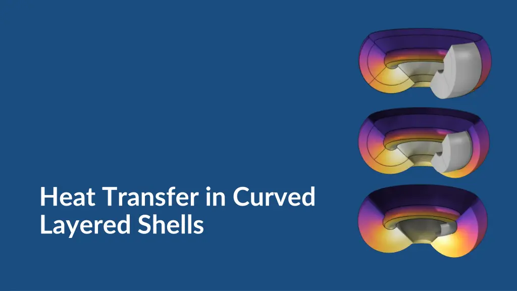
Results A stationary computation is performed to compare the three approaches. For Approach 2 and 3, the Layered Material dataset is used to visualize the temperature distribution through the steel and aluminum layers, when these layers are not explicitly represented in the geometry. Temperature distribution in the aluminum and steel layers with Approach 1 (Top), Approach 2 (Middle), and Approach 3 (Bottom)

Results The temperature results are compared with the three approaches Through the thickness of the layers Along the outer boundary The results show a very good agreement . Comparison of the temperatures with Approach 1 (solid blue lines), Approach 2 (dotted red lines), and Approach 3 (dotted green lines). Left images: through thickness plot and selection, right images: outer boundary plot and selection.