Understanding Individual Changes: A Statistical Perspective

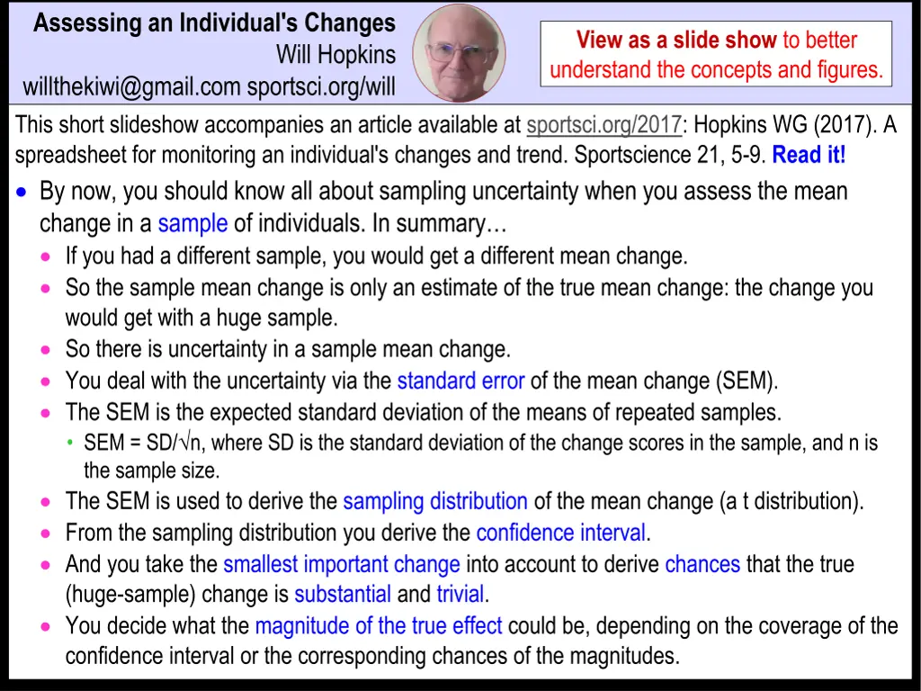
Assessing an Individual's Changes View as a slide show to better understand the concepts and figures. Will Hopkins willthekiwi@gmail.com sportsci.org/will This short slideshow accompanies an article available at sportsci.org/2017: Hopkins WG (2017). A spreadsheet for monitoring an individual's changes and trend. Sportscience 21, 5-9. Read it! By now, you should know all about sampling uncertainty when you assess the mean change in a sample of individuals. In summary If you had a different sample, you would get a different mean change. So the sample mean change is only an estimate of the true mean change: the change you would get with a huge sample. So there is uncertainty in a sample mean change. You deal with the uncertainty via the standard error of the mean change (SEM). The SEM is the expected standard deviation of the means of repeated samples. SEM = SD/ n, where SD is the standard deviation of the change scores in the sample, and n is the sample size. The SEM is used to derive the sampling distribution of the mean change (a t distribution). From the sampling distribution you derive the confidence interval. And you take the smallest important change into account to derive chances that the true (huge-sample) change is substantial and trivial. You decide what the magnitude of the true effect could be, depending on the coverage of the confidence interval or the corresponding chances of the magnitudes.

But what about uncertainty in a single change score in one individual? If you tested the individual again, you would get a different change score. Why? Because every time you measure an individual, you measure the individual's true value plus or minus random error. The random error is known as the standard error of measurement or the typical error (TE). So when you measure the individual twice, you get a change score contaminated by error of measurement in both measurements. So there is uncertainty in a single change score, which can be expressed as a standard error (SE): the expected standard deviation (SD) of repeated measurements of the change. The SE is given simply by combining the two errors of measurement: SE = SD = (TE2+TE2) = 2.TE. The calculations for confidence intervals and chances of changes are the same as for a sample of individuals. You have to assume normality of the distribution of the individual's change scores, which here is NOT guaranteed by the Central Limit Theorem. But random errors are usually pretty normal. You will need the same smallest important change as for a sample of individuals. The smallest important for a sample is actually the smallest important for individuals. If you have to use standardization to get the smallest important, the SD will have to come from a published study of a sample of individuals similar to your individual. And you will need the short-term typical error from a reliability study of similar individuals. The inference or decision or conclusion is all about the individual's true change: the change if you could somehow repeat the two tests a huge number of times and average them to get the individual's true change, free of measurement error.

A point of difference from inferences about mean change is the level of confidence for the confidence interval, and the corresponding thresholds for chances to decide whether a change has or has not occurred. For mean changes, the default is 90% confidence intervals, corresponding to >95% chance for something to be decisive (very likely) and <5% chance for something to be decisively not (very unlikely). For a single change, I recommend 80% confidence intervals, corresponding to >90% chance for decisive, and <10% for decisively not. Why? Because some measures are so noisy that many changes are indecisive with 90% intervals. But you have to live with a greater risk of error. Example: if there is a 93% chance of substantial improvement, there's a 7% chance it's not substantial. In the spreadsheets for assessing an individual's changes, I keep things simple by using non- clinical MBI, and I don't show most unlikely,unlikely, and most likely: <10% means very unlikely or decisively not a magnitude; 10-90% means possibly a magnitude (80-90% sometimes needs to be interpreted as probably); >90% means very likely or decisively a magnitude. The spreadsheets show the numeric chances, so you can interpret them how you like. You could be more conservative about the risk that the true change was harmful; e.g., <5% for decisively not harmful, rather than <10%. And with a low-enough risk of harm, you could decide that an intervention was decisively successful, even if the chance of benefit was <90%; e.g., risk of harm 3%, chance of benefit 83%.

Here are examples of each of the different outcomes with a change score, using 80% confidence intervals, and with chances and inferences as shown in the spreadsheets: Chances (%) of the true change trivial ( ) The spreadsheets do not show confidence intervals graphically. decrease ( ) increase ( ) decrease trivial increase What to tell the athlete Definitely better. Probably better. Inference 0 2 7 9 93 89 These occur rarely. 59 1 40 Could be better or similar. Definitely similar. Probably similar. 4 6 94 87 2 7 20 50 87 Could be better or worse. Could be worse or similar. Probably worse. 67 45 8 13 5 5 Definitely worse. 92 8 0 There is also a spreadsheet for recording, graphing and analyzing lots of repeated tests on an individual over an extended period. The consecutive pairwise changes are analyzed. Changes are also analyzed from one or more tests you can select as a reference. The spreadsheet also fits a straight line through selected tests to estimate a linear trend. Deviations of each test from the trend are analyzed. The mean deviation of a selected group of tests is analyzed (to improve precision). A target trend for a chosen period of time can be inserted; the spreadsheet analyzes the observed trend as an inference, with the target trend as the smallest important. The standard error of the estimate can be used as the typical error, preferably with >9 tests.

A common problem with monitoring an athlete is a high rate of indecisive changes. The rate depends partly on the magnitude of the typical error relative to the smallest important. If the error is less than half the smallest important, all changes are decisive, including zero change. Body mass is one of the few measures with negligible noise, like this. Mostly the typical error is greater the smallest important, so all trivial changes and some small substantial changes are indecisive. (Check this assertion yourself with the spreadsheet.) Example: if the test measure is time-trial time, and the time trial reproduces the demands of a race (a reasonable assumption), the smallest important is 0.3 of the athlete's variability between races; the typical error in a time trial is at least as big as the variability between races; so for time trials, the typical error is at least 1/0.3 = 3.3 greater than the smallest important. Very noisy! Hence for most tests, you should try to reduce the typical error. Where possible, you should get the athlete to repeat the test, and average the repeats: the typical error of the mean of n tests is TE/ n. Average the repeats before you put the data into the spreadsheet. Make sure you insert the appropriately smaller value for the TE. The trend spreadsheet will automatically provide an estimate of this smaller TE, with enough testing occasions (preferably >9). You might still need to use the averaging provided by the trend spreadsheet to further improve precision: average two or more tests to provide a reference value for changes; average later tests to see how they fall relative to the trend. Be prepared to give up monitoring with some tests. If most of the changes are indecisive, or if most of the changes are decisively trivial (very rare), what's the point? But the simple-change spreadsheet might show decisive one-off differences between athletes. Put one athlete's value in the first cell and the other athlete's value in the second cell.