Understanding Laplace Transform and its Applications

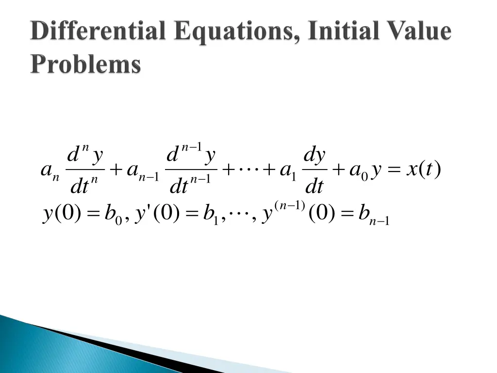
1 n n d y d y dy + + + + = ( ) a a a a y x t 1 1 0 n n 1 n n dt dt dt ) 1 = = = ( n ) 0 ( y , ) 0 ( ' y , , ) 0 ( b b y b 0 1 1 n

By Laplace Transform ( ) ) 1 1 2 ( n n n n ( s ) 1 ) 0 ( s ( ' s ) 0 n ) 0 ( ( y a + s Y s n s y s y y n ( ) 2 3 2 ) n n ( ) ) 0 ( + ( ' y = ) 0 X ) 0 ( a Y s y 1 + n ( ) + ( ) ) 0 ( ( ) ( ) a sY s y ) + a Y s s 1 0 ( X + + + s = 1 n n ( ) a s a s a Y s 1 s 0 n n ( ) ) 1 + + + + + 1 2 ( n n n ( ) ) 0 ( y ) 0 ( s a a a y Called subsidiary equation 1 1 n n

1 s = ( ) Q s Called transfer function ( ( ) + + + 1 n n a s a a 1 0 n n ) ) 1 = + + + + + 1 2 ( n n n ( ) ) 0 ( ) 0 ( R s a s a s a y y 1 1 n n The Laplace transform of y(t) ) ( s Y = + ( ) ( ) ( ) X s R s Q s y(t) is obtained by inversing the Laplace transform of Y(s)

1 t ( ) ( ) f d F s s 0 1 1 t t t 1 0 = = + st st st ( ) ( ) ( ) ( ) L f d f d e dt e f d f t e dt s s 0 0 0 0 = ( ) , 0 F s s s k s

Differentiation of transforms ( ) ( ' ) tf t F s Integration of transforms ( ) f t s d ) ( F t

( ) ( ' ) tf t F s = st ( ) ( ) F s f t e dt 0 d st ( ) f t e dt = = st 0 ( ' ) ( ) F s tf t e dt ds 0 = = st ( ) { ( )} tf t e dt L tf t 0

+ } t s sin sin t = 2 2 { ? L t d = { sin } {sin L } L t t t ds s 2 + = 2 2 2 ( ) s

( ) f t ) ( F d t s ) = st ( ) ( ) F s f t e dt 0 d s 0 ( = = t t ( ) ( ) F f t e dtd f t e d dt 0 s s s 1 t 1 t 1 t = = = t st ( ) ( ) ( ) f t e dt f t e dt L f t 0 0

2 + 1 ln 1 L 2 s 2 = + ( ) ln 1 F s 2 s 1 + 2 2 + 2 2 2 2 s + = ) 2 = = 2 3 ( ' ) 1 ( F s s 2 2 2 2 ( ) ( ) s 2 s s s s = 1 { ( ' )} 2 cos L F s t 2 2 cos t = 1 { ( )} L F s t

( ) ( ) ( ) ( ) f t g t F s G s t = st st ( ) ( ) ( ) ( ) f t g t e dt f g t d e dt 0 0 o t = = st st ( ) ( ) ( ) ( ) f g t e d dt f g t e dt d 0 0 o = = = s s s ( ) ( ) ( ) ( ) ( ) ( ) f e g e d d f e G s d F s G s 0 0 0

Integral equation t = + ( ) ( ) sin( ) y t t y t d 0 ( = t ) ? y 1 s 1 = + ( ) ( ) Y s Y s + 2 2 1 s 2 1 s s = ( ) Y s + 2 2 1 s + 2 1 1 s 1 s s = = + ( ) Y s 4 2 4 s 1 = = + 1 3 ( ) { ( )} y t L Y s t t 6

Inverse transformation of F(s) F(s) is analytic in the half plane Re{s}> m ( ) F s k | | s 1 + a j = stds ( ) ( ) f t F s e 2 i a j Called Bromwich integral formula a

+ j = = st t t ( ) ( ) ( ) F s f t e dt f t e e dt 0 0 1 j = j d at t ( ) ( ) f t e F a e 2 1 + j = + j d ( ) a t ( ) ( ) f t F a e 2 Let s=a+j ds=jd 1 + a j = stds ( ) ( ) f t F s e 2 j a j

F(s) is analytic in the s-plane except for some poles s1,s2 sn lying to the left of the vertical line Re{s}=a as Re{s} a , |s|> R0 with positive constant m, R0 and k For t>0 m s F | | = k 1 ( ) k s n = 1 st { ( )} Res F(s)e , L F s ks

1 2 = 1 ( ) L f t ) 1 + ) 2 ( ( s s st e = st ( ) F s e 2) 1 + ( 2 )( s s F(s)est has a simple pole at s=2 and a pole of order 2 at s=-1 2 ( ) t e = = st st Res[F(s)e ,2] lim s (s - 2)F(s)e 9 2 ( ) d = + st 2 st Res[F(s)e ,1] lim s e (s 1) F(s)e ds 1 st st t t ( ) 2 te s te e = = lim s 2 (s - 2) e 3 9 1 2 t t t te e = ( ) f t 9 3 9

( ) P s = ( ) F s ( ) Q s The degree of P(s) < the degree of Q(s) )} ( { s F L obtained by residue theorem 1 The degree of P(s) the degree of Q(s) ) ( ) ( 0 a a s Q ( ) P s p s = = + + + + n F s s a s 1 n ( ) ( ) q s the degree of p(s)< the degree of q(s) ) ( s q { 1 0 a s a a L + + + ( ) p s 1 L obtained by residue theorem = + + + 1 ( ) n n } ( ) ( ' ) ( ) s a t a t a t 0 1 n n

+ + 2 1 s s + = 1 ( ) L f t 2 1 s + + 2 1 s s s = = + ( ) 1 F s + + 2 2 1 1 s s 1 + = + 1 - 1 - 1 - L {F(s)} L {1} L 2 s 1 est 2 1 + = = 1 - L Res cos t + 2 s 1 s 1 = + ( ) ( ) cos f t t t

s = 1 ( ) L f t + + 2 1 s s Discuss the boundedness of f(t) for the cases =1, =-1 and =0 + 2 4 = + + = = 2 ( ) 1 0 Q s s s s 2 (1) =1 s Roots in the left side of s plane f(t) is bounded 1 i 3 = 2 (2) =-1 Roots in the right side of s plane f(t) is unbounded 1 i 3 = s 2 (3) =0 s Roots with the order of 1 are on the axis f(t) is bounded = i