Explore the differences between linear and nonlinear regression models in statistics. Linear models are expressed as straight lines or curves involving linear parameters, while nonlinear models entail complex functions not written linearly. Discover advantages and disadvantages of each type, along with insights on parameter estimation and growth functions.
Please find below an Image/Link to download the presentation.
The content on the website is provided AS IS for your information and personal use only. It may not be sold, licensed, or shared on other websites without obtaining consent from the author. If you encounter any issues during the download, it is possible that the publisher has removed the file from their server.
You are allowed to download the files provided on this website for personal or commercial use, subject to the condition that they are used lawfully. All files are the property of their respective owners.
The content on the website is provided AS IS for your information and personal use only. It may not be sold, licensed, or shared on other websites without obtaining consent from the author.
E N D
Presentation Transcript
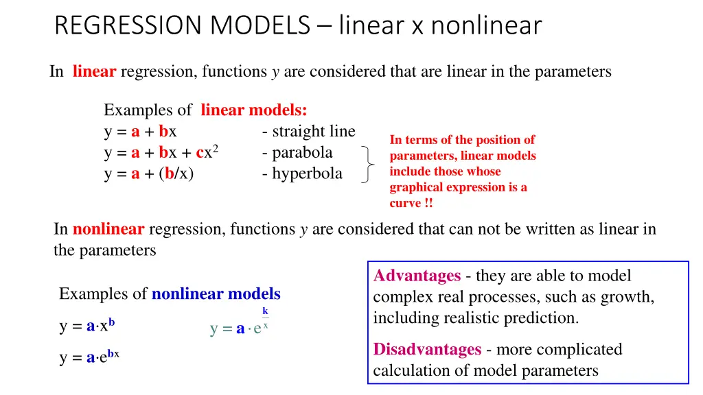
REGRESSION MODELS linear x nonlinear In linear regression, functions y are considered that are linear in the parameters Examples of linear models: y = a + bx y = a + bx + cx2 y = a + (b/x) - straight line - parabola - hyperbola In terms of the position of parameters, linear models include those whose graphical expression is a curve !! In nonlinear regression, functions y are considered that can not be written as linear in the parameters Advantages - they are able to model complex real processes, such as growth, including realistic prediction. Examples of nonlinear models k y = a xb e a y = x Disadvantages - more complicated calculation of model parameters y = a ebx
NONLINEAR MODELS ESTIMATION OF PARAMETERS Linearizable - some nonlinear regression functions can be linearized through transformation of the variable of interest and the explanatory variables. y = a xb ln(y) = ln(a) + b ln(x) = A + Bx where a = exp(A) and b = B Non-linearizable - unlike the linear regression function, when there is a system of normal equations linear leading to the function with a single minimum, in a nonlinear model the system of normal equations is nonlinear. Its solution is difficult because there is not always an unique solution and it is necessary to use iterative methods that they do not guarantee finding a global minimum of the function. Numerical methods for estimating regression parameters minimize function (sum of squares of residuals) iteratively (in consecutive steps) in order to find a solution that mathematically optimally interpolates the data. They are based on an initial estimate of the values of the function parameters.
Growth function 1. The growth function must be expressed by a mathematically justified formula. 2. It must be able to express the growth of the quantity over the whole range of age, it must be able to allow both interpolation and extrapolation, while the extrapolated values must be possible to derive from empirical values. 3. While maintaining the required flexibility, the growth function should be as simple as possible - the optimal number of calculated parameters is considered to be 2-3. 3
4. The function must be continuous, of elongated S shape. 5. At age t1it has an inflection point, until age t1it is convex from below, from age t1it is concave from below. At this point, the current (immediate) increment reaches its maximum 4
6. The growth function has an asymptote (A). It is the maximum theoretically achievable value of a growth quantity in an "infinite" age. This means that the values of the growth function approach the asymptote with increasing age, but practically never reach it. The asymptote is parallel to the t-axis. At age t2, the mean (average) increment reaches its maximum. 5
COMPARISON OF REGRESSION MODELS Akaike information criterion (AIC) RSC rezidual sum of squares m number of parameters RSS n = + ln 2 AIC n m The AIC is smaller, the model is better (from the statistical point of view!!). 7


. It is the")