Understanding Linear Equations and Systems for Problem Solving
Learn about linear equations, systems, and how to solve real-world problems using mathematical equations with simple variables. Discover the concepts through examples and visual representations.

Download Presentation

Please find below an Image/Link to download the presentation.
The content on the website is provided AS IS for your information and personal use only. It may not be sold, licensed, or shared on other websites without obtaining consent from the author. If you encounter any issues during the download, it is possible that the publisher has removed the file from their server.
You are allowed to download the files provided on this website for personal or commercial use, subject to the condition that they are used lawfully. All files are the property of their respective owners.
The content on the website is provided AS IS for your information and personal use only. It may not be sold, licensed, or shared on other websites without obtaining consent from the author.
E N D
Presentation Transcript
SYSTEM OF LINEAR EQUATION CHAPTER 2
INTRODUCTION Definition: Linear Equations a1x1+a2x2+ +anxn=ba1x1+a2x2+ +anxn=b is called a linear equation in nn variables x1,x2, ,xnx1,x2, ,xn, where ai Rai R is the coefficient of xixi, for i=1, ,ni=1, ,n and b Rb R is the constant term. x=2x=2 lis a inear equation in one variable xx. x+y=3x+y=3 is a linear equation in two variables xx and yy. x2+y=3x2+y=3 is not a linear equation. Are some examples.
A linear equation is not always in the form y = 3.5 0.5x, It can also be like y = 0.5(7 x) Or like y + 0.5x = 3.5 Or like y + 0.5x 3.5 = 0 and more. (Note: those are all the same linear equation!) A System of Linear Equations is when we have two or more linear equations working together. Example: Here are two linear equations: Together they are a system of linear equations. Can you discover the values of x and y yourself? (Just have a go, play with them a bit.) 2x x + + y y = = 5 2
Let's try to build and solve a real world example: Example: You versus Horse It's a race! You can run 0.2 km every minute. The Horse can run 0.5 km every minute. But it takes 6 minutes to saddle the horse. How far can you get before the horse catches you? We can make two equations (d=distance in km, t=time in minutes) You run at 0.2km every minute, so d = 0.2t The horse runs at 0.5 km per minute, but we take 6 off its time: d = 0.5(t 6) So we have a system of equations (that are linear): d = 0.2t d = 0.5(t 6) We can solve it on a graph:
Do you see how the horse starts at 6 minutes, but then runs faster? It seems you get caught after 10 minutes ... you only got 2 km away. Run faster next time.
Linear Equations Only simple variables are allowed in linear equations. No x2, y3, x, etc: Linear vs non-linear
Dimensions A Linear Equation can be in 2 dimensions ... (such as x and y) ... or in 3 dimensions ... (it makes a plane)
Common Variables For the equations to "work together" they share one or more variables: A System of Equations has two or more equations in one or more variables Many Variables So a System of Equations could have many equations and many variables. Example: 3 equations in 3 variables 2x + y 2z = 3 x y z = 0 x + y + 3z = 12 There can be any combination: 2 equations in 3 variables, 6 equations in 4 variables, 9,000 equations in 567 variables, etc.
Solutions When the number of equations is the same as the number of variables there is likely to be a solution. Not guaranteed, but likely. In fact there are only three possible cases: No solution One solution Infinitely many solutions When there is no solution the equations are called "inconsistent". One or infinitely many solutions are called "consistent"
The Gauss-Jordan method is similar to the Gaussian elimination process, except that the entries both above and below each pivot are zeroed out. After performing Gaussian elimination on a matrix, the result is in row echelon form, while the result after the Gauss-Jordan method is in reduced row echelon form. A homogeneous linear system is always consistent because it always has at least the trivial solution. If a homogeneous linear system has at least one nonpivot column (for example, when it has more variables than equations), then the system has an infinite number of solutions. Linear systems having the same coefficient matrix can be solved simultaneously.
This is to take Jacobis Method one step further. Where the better solution is x = (x1, x2, , xn), if x1(k+1) is a better approximation to the value of x1 than x1(k) is, then it would better that we have found the new value x1(k+1) to use it (rather than the old value that isx1(k)) in finding x2(k+1), , xn(k+1). So x1(k+1) is found as in Jacobi s Method, but in finding x2(k+1), instead of using the old value of x1(k) and old values of x3(k), , xn(k), we then use the new value x1(k+1) and the old values x3(k), , xn(k), and similarly for finding x3(k+1), , xn(k+1). This process to find the solution of the given linear equation is called the Gauss-Seidel Method The Gauss Seidel method is an iterative technique for solving a square system of n (n=3) linear equations with unknown x. Given Ax=B , to find the system of equation x which satisfy this condition. In more detail, A, x and b in their components are :
Then the decomposition of A Matrix into its lower triangular component and its upper triangular component is given by: The system of linear equations are rewritten as: The Gauss Seidel method now solves the left hand side of this expression for x, using previous value for x on the right hand side. More formally, this may be written as: However, by triangular form of L*, the elements of x(k+1) can be computed sequentially using forward substitution:
Given the three equation: 4x + y + 2z = 4 3x + 5y + z = 7 x + y + 3z = 3 First we assume that the solution of given equation is (0,0,0) Then first we put value of y and z in equation 1 and get value of x and update the value of x as (x1,0,0) Now, putting the updated value of x that is x1 and z=0 in equation 2 to get y1 and then updating our solution as (x1,y1,0) Then, at last putting x1 and y1 in equation 3 to get z1 and updating our solution as (x1,y1,z1)
An example for the matrix version A linear system shown as Ax=b is given by: We want to use the equation
Where: We must decompose A into the sum of a lower triangular component L* and a strict upper triangular component U: The Inverse of L* is:
Now we can find remaining things: Now we have T and C and we can use them to obtain the vectors x iteratively. First of all, we have to choose x{0} we can only guess. The better the guess, the quicker the algorithm will perform. We suppose:
Now we know the Exact solution which matches the answer calculated above. In fact, the matrix A is strictly diagonally dominant (but not positive definite).