Understanding Linear Homogeneous PDE with Constant Coefficients
Explore the fundamentals of linear homogeneous partial differential equations with constant coefficients, including the complementary function and particular integral. Learn to solve such equations through detailed explanations and examples for distinct cases of roots in the auxiliary equation.

Download Presentation

Please find below an Image/Link to download the presentation.
The content on the website is provided AS IS for your information and personal use only. It may not be sold, licensed, or shared on other websites without obtaining consent from the author. If you encounter any issues during the download, it is possible that the publisher has removed the file from their server.
You are allowed to download the files provided on this website for personal or commercial use, subject to the condition that they are used lawfully. All files are the property of their respective owners.
The content on the website is provided AS IS for your information and personal use only. It may not be sold, licensed, or shared on other websites without obtaining consent from the author.
E N D
Presentation Transcript
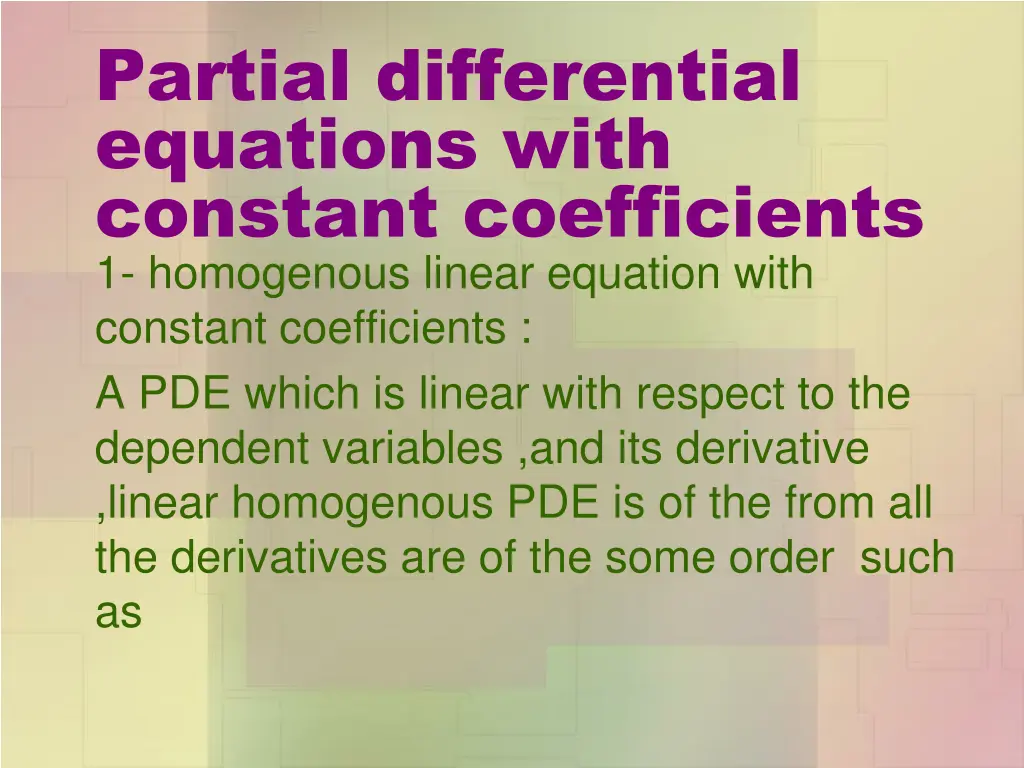
Partial differential equations with constant coefficients 1- homogenous linear equation with constant coefficients : A PDE which is linear with respect to the dependent variables ,and its derivative ,linear homogenous PDE is of the from all the derivatives are of the some order such as
??? ???+ ?1 ??? ??? ??? ??? 1??+ ?2 ??? ???= ? ?,? (1) ??? 2??2+ ?3 ??? 3??3 + .+?? ? ??,? = ? Now denote ? = ?? Then equation (1) can be written as the from (??+ ?1?? 1? + ?2?? 2? ?+ + ??? ?)? = ?(?,?)
Or ? ?,? ? = ? ?,? Solution of linear PDE Complete solution of (1) will consist of two parts a- the complementary function (C.F) b- the particular integral (P.I) the complementary function is a solution of ? ?,? ? = 0 (2)
To find the complementary function Let ? = ?(? + ??) be a the complementary function of (2) Now ??=?? ??= ?? ? + ?? ?2? ??2= ?2? (? + ??) ??? ???= ???(?)(? + ??) And ??2= Then ???=
Also ?? ??= ? ? + ?? ? ?= ?2? ??2= ? (? + ??) 2= ? ? Then ??? ???= ?(?)(? + ??) ?= ? ?
so ??? 1?? = ???(?)(? + ??) Substitution in equation (2) we get (??+ ?? 1?? 1+ .+??) ??( ) + ?? = 0 Which is satisfied if ??+ ?? 1?? 1+ .+??=0 (3) ?
the equation (4) is known as auxiliary equation The auxiliary equation obtained by putting ? = ? And ? = 1
Case1 : If ?1 ?2 ?3 .??are the distant real roots of the auxiliary equation the C.F of (1)is C.F=?1? + ?1? + ?2? + ?2? + .. ..+??? + ???
Case2 : If ?1= ?2= ?3= .= ??are the equal real roots of the auxiliary equation the C.F of (1)is C.F=?1? + ?1? + ??2? + ?2? + .. ..+????? + ???
Case 3 If ? = ? ?? are complex roots of auxiliary then C,F of equation (1) is C.F=?1? + ?1? + ?2? + ?2? + ? (?1? + ?1? ?2? + ?2? )


 is known as auxiliary")