Understanding Machine Learning Frameworks: A Visual Guide

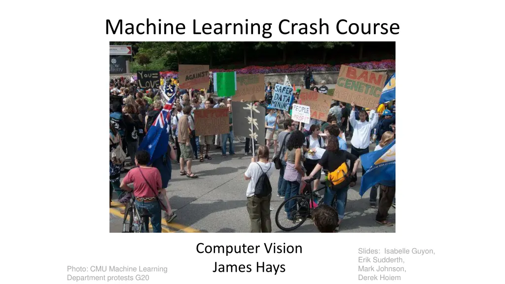
Machine Learning Crash Course Computer Vision James Hays Slides: Isabelle Guyon, Erik Sudderth, Mark Johnson, Derek Hoiem Photo: CMU Machine Learning Department protests G20

The machine learning framework Apply a prediction function to a feature representation of the image to get the desired output: f( ) = apple f( ) = tomato f( ) = cow Slide credit: L. Lazebnik

Learning a classifier Given some set of features with corresponding labels, learn a function to predict the labels from the features x x x x x x x o x o o o o x2 x1

Generalization Training set (labels known) Test set (labels unknown) How well does a learned model generalize from the data it was trained on to a new test set? Slide credit: L. Lazebnik

Very brief tour of some classifiers K-nearest neighbor SVM Boosted Decision Trees Neural networks Na ve Bayes Bayesian network Logistic regression Randomized Forests RBMs Deep Convolutional Network Attentional models or Transformers Etc.

Classification Assign input vector to one of two or more classes Any decision rule divides input space into decision regions separated by decision boundaries Slide credit: L. Lazebnik

Nearest Neighbor Classifier Assign label of nearest training data point to each test data point from Duda et al. Voronoi partitioning of feature space for two-category 2D and 3D data Source: D. Lowe

K-nearest neighbor x x o x x x x + o x o x + o o o o x2 x1

1-nearest neighbor x x o x x x x + o x o x + o o o o x2 x1

3-nearest neighbor x x o x x x x + o x o x + o o o o x2 x1

5-nearest neighbor x x o x x x x + o x o x + o o o o x2 x1

Using K-NN Simple to implement and interpret, a good classifier to try first

Classifiers: Linear SVM x x x x x x x o x o o o o x2 x1 Find a linear function to separate the classes: f(x) = sgn(w x + b)

Classifiers: Linear SVM x x x x x x x o x o o o o x2 x1 Find a linear function to separate the classes: f(x) = sgn(w x + b)

Classifiers: Linear SVM x x o x x x x x o x o o o o x2 x1 Find a linear function to separate the classes: f(x) = sgn(w x + b)

Nonlinear SVMs Datasets that are linearly separable work out great: x 0 But what if the dataset is just too hard? x 0 We can map it to a higher-dimensional space: x2 0 x Slide credit: Andrew Moore

Nonlinear SVMs General idea: the original input space can always be mapped to some higher-dimensional feature space where the training set is separable: : x (x) Slide credit: Andrew Moore

Nonlinear SVMs The kernel trick: instead of explicitly computing the lifting transformation (x), define a kernel function K such that K(xi,xj) = (xi ) (xj) (to be valid, the kernel function must satisfy Mercer s condition) This gives a nonlinear decision boundary in the original feature space: ) ( ) ( i + = + x x x x ( , ) y b y K b i i i i i i i C. Burges, A Tutorial on Support Vector Machines for Pattern Recognition, Data Mining and Knowledge Discovery, 1998

Nonlinear kernel: Example x = 2 Consider the mapping ( ) ( , ) x x x2 = = + 2 2 2 2 ( ) ( ) ( , ) ( , + ) x y x x y y xy x y = 2 2 ( , ) K x y xy x y

State of the art in 2007: Kernels for bags of features Histogram intersection kernel: N = i = ( , ) min( ( ), ( )) I h h h i h i 1 2 1 2 1 Generalized Gaussian kernel: 1 A = 2 ( , ) exp ( , ) K h h D h h 1 2 1 2 D can be (inverse) L1 distance, Euclidean distance, 2 distance, etc. J. Zhang, M. Marszalek, S. Lazebnik, and C. Schmid, Local Features and Kernels for Classifcation of Texture and Object Categories: A Comprehensive Study, IJCV 2007

Summary: SVMs for image classification 1. Pick an image representation (e.g. histogram of quantized sift features) 2. Pick a kernel function for that representation 3. Compute the matrix of kernel values between every pair of training examples 4. Feed the kernel matrix into your favorite SVM solver to obtain support vectors and weights 5. At test time: compute kernel values for your test example and each support vector, and combine them with the learned weights to get the value of the decision function Slide credit: L. Lazebnik

What about multi-class SVMs? Unfortunately, there is no definitive multi-class SVM formulation In practice, we have to obtain a multi-class SVM by combining multiple two-class SVMs One vs. others Traning: learn an SVM for each class vs. the others Testing: apply each SVM to test example and assign to it the class of the SVM that returns the highest decision value One vs. one Training: learn an SVM for each pair of classes Testing: each learned SVM votes for a class to assign to the test example Slide credit: L. Lazebnik

SVMs: Pros and cons Pros Linear SVMs are surprisingly accurate, while being lightweight and interpretable Non-linear, kernel-based SVMs are very powerful, flexible SVMs work very well in practice, even with very small training sample sizes Cons No direct multi-class SVM, must combine two-class SVMs Computation, memory During training time, must compute matrix of kernel values for every pair of examples. Quadratic memory consumption. Learning can take a very long time for large-scale problems

Very brief tour of some classifiers K-nearest neighbor SVM Boosted Decision Trees Neural networks Na ve Bayes Bayesian network Logistic regression Randomized Forests RBMs Deep Convolutional Network Attentional models or Transformers Etc.

Generalization Training set (labels known) Test set (labels unknown) How well does a learned model generalize from the data it was trained on to a new test set? Slide credit: L. Lazebnik

Generalization Components of generalization error Bias: how much the average model over all training sets differ from the true model? Error due to inaccurate assumptions/simplifications made by the model. Bias sounds negative. Regularization sounds nicer. Variance: how much models estimated from different training sets differ from each other. Underfitting:model is too simple to represent all the relevant class characteristics High bias (few degrees of freedom) and low variance High training error and high test error Overfitting:model is too complex and fits irrelevant characteristics (noise) in the data Low bias (many degrees of freedom) and high variance Low training error and high test error Slide credit: L. Lazebnik

Bias-Variance Trade-off Models with too few parameters are inaccurate because of a large bias (not enough flexibility). Models with too many parameters are inaccurate because of a large variance (too much sensitivity to the sample). Slide credit: D. Hoiem

Bias-variance tradeoff Underfitting Overfitting Error Test error Training error High Bias Low Variance Low Bias High Variance Complexity Slide credit: D. Hoiem

Bias-variance tradeoff Few training examples Test Error Many training examples High Bias Low Variance Low Bias High Variance Complexity Slide credit: D. Hoiem

Effect of Training Size Fixed prediction model Error Testing Generalization Error Training Number of Training Examples Slide credit: D. Hoiem

Remember No classifier is inherently better than any other: you need to make assumptions to generalize Three kinds of error Inherent: unavoidable Bias: due to over-simplifications / regularization Variance: due to inability to perfectly estimate parameters from limited data Slide credit: D. Hoiem

How to reduce variance? Choose a simpler classifier Regularize the parameters Get more training data How to reduce bias? Choose a more complex, more expressive classifier Remove regularization (These might not be safe to do unless you get more training data) Slide credit: D. Hoiem

What to remember about classifiers No free lunch: machine learning algorithms are tools, not dogmas Try simple classifiers first Better to have smart features and simple classifiers than simple features and smart classifiers Use increasingly powerful classifiers with more training data (bias- variance tradeoff) Slide credit: D. Hoiem

Machine Learning Considerations 3 important design decisions: 1) What data do I use? 2) How do I represent my data (what feature)? 3) What classifier / regressor / machine learning tool do I use? These are in decreasing order of importance Deep learning addresses 2 and 3 simultaneously (and blurs the boundary between them). You can take the representation from deep learning and use it with any classifier.

Andrew Ngs ranking of machine learning impact 1. Supervised Learning 2. Transfer Learning 3. Unsupervised Learning (I prefer self- supervised learning) 4. Reinforcement Learning James thinks 2 and 3 might have switched ranks.