Understanding Multivariate Methods for Data Analysis

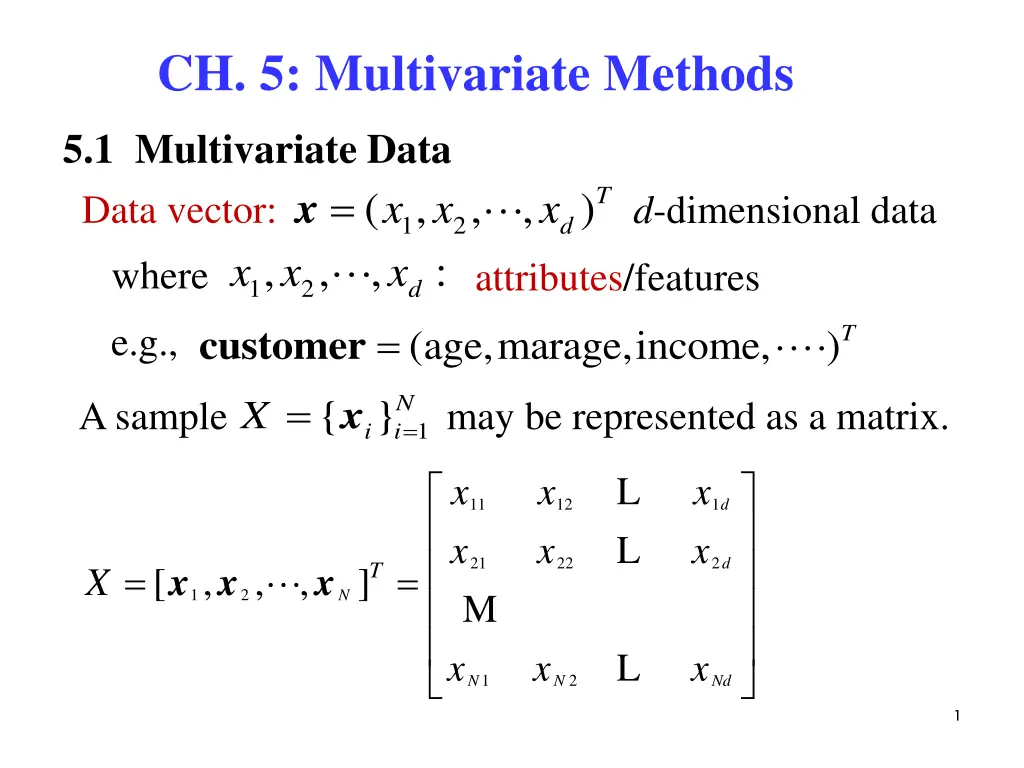
CH. 5: Multivariate Methods 5.1 Multivariate Data Data vector: x x where = )T x ( , x x , d x = , , x d-dimensional data 1 2 d , , : attributes/features 1 2 e.g., )T customer (age,marage,income, A sample may be represented as a matrix. 1 { }N i i X = = x L L x x x x x x 11 12 1 d 21 M 22 2 d = , , = T x x x [ , ] X 1 2 N L x x x 1 2 N N Nd 1

5.2 Parameter Estimation x T = = Mean vector: 1, , , E d = E x N = where p x i i ij ij = 1 j Covariance matrix: [( E x covariance of 2 1 L L 12 2 2 1 d ( )( ) T = = 21 M 2 d x x E 2 d L where 1 2 d d = = = = 2 i 2 ix Var( ) Cov( , [( = ) ] : x E x ) j variance of i i i )( )] x x x ij i i i j j and x x [ ] : E x x i j i j i j 2

Correlation coefficient: ( ) Cov , x x ( ) i j ij = = = Corr , x x ij i j Var( ) Var( i x ) x i j j Parameter Estimation { }N i i = x ( m m = X Given a sample = = N 1 , , x ij = 1 j m Sample mean: , ), m m 1 2 d i N Sample covariance matrix: )( ) = ( N x m N [ ], ij r x m ik i jk j = = 1 [ ], where ij s k S s ij s = = ij R r Sample correlation matrix: ij s s i j 3

5.3 Estimation of Missing Values Certain instances have missing attributes. Ignore those instances: not a good idea if the sample is small. Imputation: Fill in the missing value Mean imputation: Substitute the mean of the available data of the missing attribute Imputation by regression: Predict based on other attributes 4

5.4 Multivariate Normal Distribution ( ) = T x Suppose data vector ( , x x , , ) ~ , x N 1 2 d 1 d 1 2 ( ) x ( ) ( ) T = 1 x x i.e., exp p ( ) /2 1/2 ) 2 ( ( ) T 1 where x x : Mahalanobis distance measures the distance from x to in terms of , which normalizes variances of different dimensions 5

e.g., ( ) 2 x 1 ( ) p x = exp d = 1, ( ) 1/2 2 2 2 ( ) 2 2 x the square distance from x to in unit. x ( ) ( ) = = 2 1 ( ) : x x 2 2 1 2 1 = = 12 2 2 1 2 d = 2, 2 2 12 1 2 2 1 = = = 2 1 2 2 2 2 1 2 2 2 2 1 2 2 1 2 (1 ) 2 2 1 2 6

2 2 2 2 1 2 1 2 1 2 1 2 2 2 = = 1 1 2 1 2 2 2 1 (1 ) 1 2 1 1 1 2 = 2 1 1 2 2 1 2 1 2 1 1 ( ) ( ) ( ) ( ) T T 1 2 1 x x x x = 2 1 1 2 2 1 2 7

1 2 1 x x 1 1 2 1 1 = ( ) x x 1 1 2 2 2 1 1 2 2 2 2 1 2 2 2 1 x x x x = + 2 1 1 1 1 2 2 2 2 2 1 1 1 2 2 x (z- normalization) = = , 1,2 z i i i Let i i 1 ( ) ( ) ( ) T = + 1 2 1 2 2 x x 2 z 1 2 z z z 2 1 + = 2 1 2 2 2 2 . z 1 2 z z z c Consider 8

the above equation expresses an ellipse. For 1, the major axis of the ellipse has a positive (negative) slope. 0 ( 0), When 9

10

( ) ( ) T . 1 : hyperellipsoid centered at = 1 2 x x c Both its shape and orientation are governed by , which normalizes all variables to their unit standard deviations. ( ) ~ , , . x w N R [ ] [ ] E E = = w x w x w Q ( ) d T T T w x . w w w ~ , N Let ( T T T = 2 T T T w x w x w x w Var( = = ) [( w x [ ]) ] x w E E = 2 T T T T w x x w w [( ) ] [( w ( )( ) ] E w E = T T T x [( )( ) ] ) E i.e., The projection of a d-D normal on a vector w is univariate (i.e., 1-D) normal. 11

W be a matrix. d k Let ( ) T T T x Then ~ , : variate normal W N W W W k 5.5 Multivariate Classification i C From the Bayes rule, the posterior probability of ( | ) ( ( | ) ( ) p x Define discriminant function of ( ) ( ) log | log i i g p C = + x x x ) p C p C 1, , = = i K x , P C i i i i C ( ) . P C i Assume ( | p x 1 1 2 ) ( ) ( ) T = 1 x x exp C ( ) i i i i /2 1/2 d 2 i 12

1 2 ---- (A) 1 2 d ( ) ( ) ( ) x T = 1 x x log2 log g i i i i i 2 log ( ) + P C i { , } , = x r t t N t Given a sample X where = 1 x 1 0 C = = = i x r { , x , }, { , r , }, x r r 1 1 d K i otherwise ( ), , P C Estimation of Parameters i i i ( )( t i r ) = T t t t x m x m t t t x r r r ( ) i i i i i = = m t , , P C S t t i i i t N r i t t d log2 Substituting into (A) and ignore 2 13

1 2 1 2 log 1 2 1 2 ( ( ) ( ) ( ) ( ) x T = + 1 x m x m log log g S S P C i i i i i i ) = + 1 1 1 T T T x x x m m m log 2 S S S S i i i i i i i ( ) + ----- (B) P C i ( ) x = + + T T x x w x i g W w i) Quadratic discriminant: 0 i i i 1 2 1 2 = = 1 1 w m where , W S S i i i i 1 2 i ( ) = + 1 T m m log log w S S P C 0 i i i i i i The number of parameters to be estimated is for means and for covariance matrices S K d 1)/2 , . K = m Kd d + , i = ( , , , ) m m m ( 1 2 i d = [ ] 1, mn d d s i 14

= Share common sample covariance, and 1log S 1 x x m x i i g S = i.e., , i S S i ignore . (B) reduces to 2 ( ) ( 2 ) ( ) ( ) T + 1 m log P C i i 1 2 ( ) ( ) P C = + 1 1 1 T T T x x x m m m 2 +log -- (C) S S S i i i i K d The numbers of parameters to be estimated: for means and for covariance matrices. ( 1)/2 d d + TS Ignoring quadratic term , (C) reduces to 1 2 1 x x ( ) ( ) x = + 1 1 T T x m m m log ---- (D) g S S P C i i i i i 15

( ) x = + T w x g w ii) Linear discriminant: 0 i i i 1 2 ( ) = = + 1 1 T w m m m where , log S w S P C 0 i i i i i i Assuming off-diagonals of S to be 0, 1/ 2 1 0 2 1 0 s 0 0 0 s s 2 2 2 2 0 1/ s = = 1 and S S 0 s 0 2 d 2 d 0 0 0 0 1/ s 1 2 ( ) ( ) T S Substitute into 1 x m x m i i 16

1/ 2 1 0 0 s 2 2 0 1/ s 1( 2 = , , , ) g x m x m x m 1 1 2 2 i i d di 0 2 d 0 0 1/ s x x m m 1 1 i 2 x m d 1 2 2 2 i j ij = g s = 1 j j x m d di Substitute this into (C) 17

iii) Naive Bayes classifier: 2 x m d 1 2 ( ) ( ) x j ij = + log ---- (E) g P C i i s = 1 j j The number of parameters to be estimated is for means and d for covariance matrices. K d = Assuming all variances to be equal, i.e., j s s j d 1 s ( ) 2 ( ) ( ) x = + t j (E) log g x m P C i ij i 2 2 = 1 j K d The number of parameters to be estimated is for means and 1 for . 2s 18

( ) Assuming equal priors and ignore s, ( 1 j = iv) Nearest mean classifier: ( ) ( 2 xx m x+ m m i = P C i d ) 2 ( ) x 2 = = t j x m g x m i ij i 2 = = T x x m x m x m ( ) ( ) g i i i i T T T ) i i xxT m x = Ignore the common term 1 2 1 2 ( ) x 2 = T T T m x i m m i m g i i i i mi Assuming equal , ( ) x = T m x g v) Inner product classifier: i i 19

5.6 Tuning Complexity As we increase complexity, bias decreases but variance increases (bias-variance dilemma). 20

5.7 Discrete Attributes = ( , , , ), x x x x Binary features: 1 2 d jx where are binary. {0, 1} ( ) ( ) ( ) ( ) 1 x x ij = = = j | 1 Let 1 | . p x C p p p p x C j j i ij ij j i If xj s are independent, ( ) d d ( ) ( ) ( ) 1 x x ij = = x j | | 1 p C p x C p p j i j i ij = = 1 1 j j The discriminant function: ( ) ( ) P C ( ) x = + x log | log g p C i i i ( ) ( ) ( ) P C = + + log 1 log 1 log x p x p j ij j ij i j 21

= ( , , , ), x x x x Multinomial features: 1 2 d = 1 0 if otherwise x v { , , , v v } x v = j k z 1 2 j n Define j jk Let : the probability that takes value , ijk p ( 1| ijk jk i p p z C p x = = = x C kv j i ) ( ) = | v C i.e., j k i n d d ( ) j ( ) z ijk = = x | | p C p x C p If xj s are independent, jk i j i = = = 1 1 1 j j k The discriminant function: ( ) log i g p x x n d j ( ) ( ) P C ( ) P C z ijk = + = + | log log log C p jk i i i = = 1 1 j k ( ) P C = + log log z p jk ijk i j k 22

5.8 Multivariate Regression Linear multivariate model ( ) = + t t x | , ,..., r f w w w 0 1 d + = + + + + t t t d L w w x w x w x 0 1 1 2 2 d 2 ~ (0, ) Assume N Then, maximizing the likelihood minimizing the sum of squared error 2 N 1 2 ( ) = t t t d , ,..., | L E w w w X r w w x w x 0 1 0 1 1 d d = 1 w w t , ,..., w Taking derivatives wrt , respectively, 0 1 d 23

= + + + + t t t t d r Nw w x w x w x 0 1 1 2 2 d t t t t = + + + + 2 t t t t t t t t d ( ) x x r w x w w x x w x x 1 0 1 1 1 2 1 2 1 d t t t t t = + + + + 2 t d t t d t d t t t t d ( ) x r w x w x x w x x w x 0 1 1 2 1 2 d t t t t t = T T r w In vector-matrix form: , where X = ( ) X X = w X X 1 1 2 1 1 d 1 1 x x x = w w 1 r r 0 2 1, X , X = = w r . N N d 1 x x w N r 1 d + 1 T T r r X Solution: 24

Generalizing the linear model: i) A polynomial model can lead to a linear multivariate , x x = = = 2 k , , x x x x model by letting 1 2 k Example: Find a quadratic model of two variables and , i.e., x w w x + x 1 2 = + + + + 2 2 ( , ) f x x w x 3 1 2 w x x w x w x 1 2 0 1 1 2 2 4 1 5 2 to fit a sample = = t t t N t x ( ( , x x ), ) , r X = 1 2 1 i.e., determine iw i = , 1, ,5. Answer: Write the fit as = + + + + + ( , ) f x x w w z w z w z w z w z 1 2 0 1 1 2 2 3 3 4 4 5 5 25

= = = = = 2 1 2 2 , , , , z x z x z 1 2 x x z x z x where 1 1 2 2 3 4 5 i w i = , 1, ,5. Use linear regression to learn = = 2 ii) Let sin , exp , x x x x 1 2 A nonlinear model can lead to a linear multivariate model. 26

Summary Multivariate methods -- deal with multivariate data. = )T x , ( , x x , d x , , x Multivariate data: where 1 2 d , : x x attributes/features 1 2 Multivariate parameters of interest: x T = = Mean vector: 1, , , E d = E x N = where p x i i ij ij = 1 j 27

Covariance matrix: 2 1 L L 12 2 2 1 d ( )( ) T = = 21 M 2 d x x E 2 d L 1 2 d d = = where 2 i 2 Var( ) [( ) ] : x E x i i i = = = Cov( , ) [( )( )] x x E x x ij i j i i j j [ ] : E x x i j i j ij = Correlation matrix: , were ij ij i j 28

Imputation: estimating missing values Mean imputation: Substitute the mean of the available data of the missing attribute Imputation by regression: Predict based on other attributes Multivariate Normal Distribution 1 1 2 ( ) x ( ) ( ) T = 1 x x exp p ( ) /2 1/2 d 2 29

( ) ( ) T Mahalanobis distance 1 x x : measures the distance from x to which normalizes variances of different dimensions. in terms of , ( . ) ( ) T : hyperellipsoid centered at = 1 2 x x c Both its shape and orientation are governed by , which normalizes all variables to their unit 1 standard deviations. ~ x N ( ) ( ) d w , , . R T T T w x w w w Let ~ , N i.e., The projection of a d-D normal on a vector w is univariate (i.e., 1-D) normal. 30

W be a matrix. d Let k ( ) T T T x Then ~ , : variate normal W N W W W k Multivariate Classification ( ) x = + + T T x x w x i i) Quadratic discriminant: g W w 0 i i i 1 2 1 2 = = 1 1 w m where , W S S i i i i 1 2 i ( ) = + 1 T m m log log w S S P C 0 i i i i i i ( ) x = + T w x g w ii) Linear discriminant: 0 i i i 1 2 ( ) = = + 1 1 T w m m m where , log S w S P C 0 i i i i i i 31

iii) Naive Bayes classifier: 2 x m d 1 2 ( ) ( ) x j ij = + log ---- (E) g P C i i s = 1 j j iv) Nearest mean classifier: ( ) ( 2 xx = 2 = = T x x m x m x m ( ) ( ) g i i i i T T T m x+ m m i ) i i ( ) x = T m x g v) Inner product classifier: i i 32

33