Explore the fundamentals of numerical differentiation and integration in calculus, essential for dealing with systems that involve continuous change. Learn about derivatives, integrals, and their inverse relationship, as well as methods for differentiation and integration.
Please find below an Image/Link to download the presentation.
The content on the website is provided AS IS for your information and personal use only. It may not be sold, licensed, or shared on other websites without obtaining consent from the author. If you encounter any issues during the download, it is possible that the publisher has removed the file from their server.
You are allowed to download the files provided on this website for personal or commercial use, subject to the condition that they are used lawfully. All files are the property of their respective owners.
The content on the website is provided AS IS for your information and personal use only. It may not be sold, licensed, or shared on other websites without obtaining consent from the author.
E N D
Presentation Transcript
NUMERICAL DIFFERENTIATION AND INTEGRATION Prof. Samuel Prof. Samuel Okolie Adekunle Adekunle & Dr. Okolie, Prof. & Dr. Seun Seun Ebiesuwa , Prof. Yinka Ebiesuwa Yinka
Calculus is the mathematics of change. Because scientists and engineers must continuously deal with systems and process that change, calculus is an essential tool. Standing at the heart of calculus are the related mathematical concepts of differentiation and integration. Mathematically the derivative, which serves as the fundamental vehicle for differentiation, represents the rate of change of a dependent variable with respect to an independent variable. The mathematical definition of derivation begins with a difference approximation: ? ?= f (x + x) f(x ) x (divided difference)
Where y and f(x) are alternative representation for the dependent variable, and x is the independent variable. If x is allowed to approach o, the difference becomes a derivative. ?? ?? = lim f (x + x) f(x) = f/ (x) = y/ x 0 x y f(x + x) f(x) tangent y f(x ) x x x + x x
As x decreases i.e 0, the difference becomes a derivative (1st derivative). The inverse process of differentiation in calculus is integration. Mathematically integration is represented by ? 1 = ?(?) ? dx is a sylised capital S which stands for the integral ( summation ) of the function f(x) with respect to x, evaluated between the limits x = a to x = b. The function f(x) is called the integrand
f(x) a b x graphical representation of the integral of f(x) between the limits x = a and x = b. The integral is equivalent to the area under the case of definite integration. When the limits of a and b are not specified it is indefinite integration. Integration and differentiation are inversely related thus, we can make the general claim that the evaluation of the integral ? 1 = ?(?) ? dx is equivalent to solving the differential equation ?? ?? = f(x) for y(b) given the initial condition y(a) = 0
Non computer Methods for Differentiation and Integration The functions to be differentiated or integrated will typically be in one of the following three forms: (1)A simple continuous function such as a polynomial, an exponential, a trigonometrically or logarithmic function. (2)A complicated continuous function that is different or impossible to differentiate or integrate directly. (3)A tabulated function where values of x and f(x) are given at discrete points as in the case of experimental or fields data.
In the first case the derivative or integral of a simple function may be evaluated analytically using calculus. For the second case, analytical solution are often impractical and sometimes impossible, to obtain. In this case approximate numerical methods must be employed. For the third case of discrete data, approximate method must be employed. A non-computer method, the (x, y) data are tabulated and, for each interval, a simple divided difference ?/ ? is employed to estate the slope. Then these values are plotted as a stepped curve Vs x.
Next, a smooth curve is draw that attempts to approximate the area under the stepped curve. That is, it is drawn so that visually the negative and the positive areas are balanced. The rates at given values of x can then be read from the curve. X y ?/ ? 0 0 66.7 66 .7 3 200 50 6 350 40 50 9 470 30 15 650 23.5 30 18 720 10 The derivative estimate are plotted as a bar graph . 3 6 9 12 15 18 A smooth curve is EQUAL AREA DIFFERENTIATION Superimposed on the plot to approximate the area under the bar graph. x 0 3 6 9 15 18 Read from the curve at given values of x. dy/dx 76.50 57.50 45.00 36.25 25.00 12.50
In a similar manner, numerical integration methods are available to obtain integrals. These methods are easier to implement than the grid method and are similar in spirit to the strip method. That is, function heights are multiplied by strip widths and summed to estimate the integral. As in the simple strip method, numerical integration and differentiation techniques utilize data at discrete points because tabulated information is already in such a form, it is naturally compatible with many of the numerical approaches. Although, continuous functions are not originally in discrete form, it is usually a simple proportion to use the given equation to generate a table of values. This table can then be evaluated with a numerical method.
points discrete continuous function 2 1 0 0 Mathematical Background for differentiation and Integration Basic general differentiation methods using calculus Some simple integral to be noted. Use of strip (rectangular) method to estimate the the integral on the basis of the discrete points. 0.5 1 1. 5 2.0 x These are the subject of the introductory module titled differentiation and integration.


 are alternative representation for the")

")