Understanding Probability and Random Variables in Statistics Review

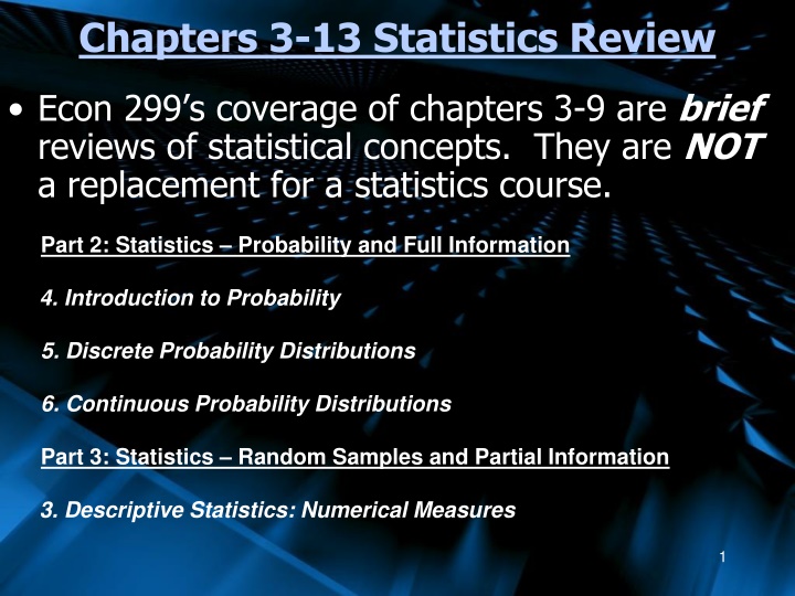
Chapters 3-13 Statistics Review Econ 299 s coverage of chapters 3-9 are brief reviews of statistical concepts. They are NOT a replacement for a statistics course. Part 2: Statistics Probability and Full Information 4. Introduction to Probability 5. Discrete Probability Distributions 6. Continuous Probability Distributions Part 3: Statistics Random Samples and Partial Information 3. Descriptive Statistics: Numerical Measures 1

Chapter 4 Introduction to Probability By the end of the chapter, you will be able to: 1) Understand probability definitions 2) Understand and use probability rules 3) Work with marginal probabilities 4) Work with joint probabilities 5) Work with conditional probabilities 6) Recognize statistically (in)dependent events 7) Become a better human being 2

4.1 Probability Definitions Experiment A process that generates one or more well-defined outcomes ex) Rolling a die ex) Taking a test ex) Measuring your height ex) Employment survey Some outcomes can be more likely than others (ie: greater chance to pass an exam than fail, more likely to roll an 8 than a 5) 3

4.1 Probability Definitions Random Variable A variable whose value is determined by the outcome of a experiment ex) Sum of the dice roll ex) Passing or Failing an exam ex) How tall you are ex) Employment Status 4

4.1 Probability Definitions Outcome Any result of an experiment ex) A roll of 9 (on 2 6-sided die) ex) Passing an exam ex) A height of 177cm ex) Unemployed (Referred to in the text as a sample point. Sometimes referred to as an observation.) 5

4.1 Random Variables Discrete Variable Can take on a finite # of values Ie: Dice roll, card picked Continuous Variable Can take on any value within a range Ie: Height, weight, time Variables are often assumed discrete to aid in calculations and economic assumptions (ie: Money in increments of 1 cent) 6

4.1 Probability Terminology Sample Space Set of all possible outcomes from a random experiment -ex) S = {2, 3, 4, 5, 6, 7, 8, 9, 10, 11, 12} -ex) E = {Pass exam, Fail exam, Fail horribly} Event A subset of the sample space -ex) B = {3, 6, 9, 12} S -ex) F = {Fail exam, Fail horribly} E 7

4.1 Quiz Example Students do a 4-question quiz with each question worth 2 marks (no part marks). Handing in the quiz is worth 2 marks, and there is a 1 mark bonus question. Events: -getting a zero (not handing in the quiz) -getting at least 40% (at least 1 right) -getting 100% or more (all right or all right plus the bonus question) -getting 110% (all right plus the bonus question) *Events contain one or more possible outcomes 8

4.1 Probability Probability = the likelihood of an event occurring (between 0 and 1) P(a) = Prob(a) = probability that event a will occur P(Y=y) = probability that the random variable Y will take on value y P(ylow < Y < yhigh) = probability that the random variable Y takes on any value between ylow and yhigh 9

4.1 Probability Examples P(true love) = probability that you will find true love P(Sleep=8 hours) = probability that the random variable Sleep will take on the value 8 hours P($80< Wedding Gift < $140) = probability that the random variable Wedding Gift takes on any value between $80and $140 10

4.1 Probability Calculations IF probability can be calculated, two methods are: ) ( a P # of outcomes including a = # of outcomes total # of outcomes including a = ( ) P a # of trials -Method 1 is used for full information (die roll) -Method 2 is used for a test (asking names at a party) 11

4.1 Probability of Small Worlds Die In the board game Small World, the 6-sided die has a blank (0) on 3 sides, and a 1, 2, and 3 on each of the remaining sides 3 ) 0 ( = P P 1 = ) 2 ( 6 6 1 1 = = ) 1 ( P ) 3 ( P 6 6 12

4.1 Probability Extremes If Prob(a) = 0, the event will never occur ie: Canada moves to Europe ie: the price of cars drops below zero ie: your instructor turns into a giant llama If Prob(b) = 1, the event will always occur ie: you will get a mark on your final exam ie: you will either marry your true love or not ie: the sun will rise tomorrow 13

4.2 Probability Terminology Mutually Exclusive Events cannot occur at the same time -rolling both a 3 and an 11; being both dead and alive; Exhaustive Events cover all possible outcomes -a dice roll must lie within S [2,12] -a person is either married or not married Complement everything other than the event -being dead is the complement to being alive -rolling an 11 or 12 is a complement to rolling a 2, 3, 4, 5, 6, 7, 8, 9, or 10 14

4.2 Probability Rules 1) Probability Range P(a) must be greater than or equal to 0 and less than or equal to 1 : 0 P(a) 1 2) Something Must Happen P(a) =1 15

4.2 Probability Rules 3) Exhaustive Rule If any set of events (ie: {A,B,C}) are exhaustive, then P(A or B or C) = 1 ex) Prob(winning, losing or tying)=1 4a) Addition Rule (Mutually Exclusive) If any set of events (ie: {A,B,C}) are mutually exclusive, then P(A or B or C)=P(A)+P(B)+P(C) ex) Prob. of marrying the person to the right or left 16

4.2 Probability Rules 4b) Addition Rule (General) P(A or B)=P(A)+P(B)-P(A+B) Example: P(Marrying a fellow student OR someone named Joe) = P(Marry a fellow student) +P(Marry Joe) -P(Marry a fellow student named Joe) 17

4.2 Probability Rules 5) Complement Rule P(not A) = P(Ac) = 1-P(A) Example: P(Not eating ice cream)=1-P(Eating Ice Cream) 6) Multiplication Rule(A and B are independent/unrelated) P(A and B)=P(A)P(B) Example: P(Owning a cat AND having black hair) =P(Owning a Cat)P(Having black hair) 18

4.3 Union (or) The probability of event A or event B occurring is often referred to as the probability of A union B: ? ? ?? ? = ?(? ?) ? ? ?(? ?) 19

4.3 Intersection (and) The probability of event A and event B occurring is often referred to as the probability of A intersection B: ? ? ??? ? = ?(? ?) ?(? ?) ? ? 20

4.2 Probability of Small World I have the last moves in Smallworld. Colin has 81 points, and I have 80. (If our points are tied, I win.) I have 3 final attacks with the die. I lose each attack on a roll of zero, otherwise I win. Each attack I win gets me one point. What is the probability that I will win and Colin will lose? 21

4.2 Probability of Small World 3 1 = = ) 0 ( P ) 2 ( P 6 6 1 1 = = ) 1 ( P ) 3 ( P 6 6 = ( ) 1 ( ) P Win P Lose = ( ) 1 { ( 1 ) ( 2 ) 3 )} P Win P Lose st P Lose nd PLose rd = ( ) 1 5 . 0 ( 5 . 0 ) 5 . 0 {( )} P Win = ( ) 1 . 0 125 P Win = ( ) . 0 875 P Win 22 There is an 87.5% chance that I will win.

4.2 Probability Examples 1) P(coin flip=heads) = 2) P(2 coin flips=2 heads) = 3) Probability of tossing 6 heads in a row = 1/64 4) Probability of rolling less than 4 with 1 six- sided die = 3/6 5) Probability of throwing a 13 with 2 dice= 0 6) Probability of winning rock, paper, scissors = 1/3 (or 3/9) 7) Probability of being in love or not in love=1 8) Probability of passing the course = ? 23

4.2.1 Probability Density Functions The probability density function (pdf) summarizes probabilities associated with possible outcomes Discrete Random Variables pdf f(y) = Prob (Y=y) f(y) = 1 -(the sum of the probabilities of all possible outcomes is one) 24

4.2.1 Dice Example The probabilities of rolling a number with the sum of two six- sided die Each number has different die combinations: 7={1+6, 2+5, 3+4, 4+3, 5+2, 6+1} Exercise: Construct a table with one 4-sided and one 8-sided die y f(y) y f(y) 2 1/36 8 5/36 3 2/36 9 4/36 4 3/36 10 3/36 5 4/36 11 2/36 6 5/36 12 1/36 7 6/36 25

4.2.1 Probability Density Functions Continuous Random Variables pdf f(y) = pdf for continuous random variable Y f(y)dy = 1 (sum/integral of all probabilities of all possibilities is one) -probabilities are measured as areas under the pdf, which must be non-negative -technically, the probability of any ONE event is zero 26

4.2.1 Continuous EXAMPLE Continuous Random Variables pdf f(y) = 0.2 for 2<y<7 = 0 for y <2 or y >7 f(y) = 3 y 7 = = = = 7 3 3 ( P ) 7 2 . 0 2 . 0 [ ] ) 7 ( 2 . 0 ) 3 ( 2 . 0 8 . 0 Y dy y This course will ALWAYS assume variables are DISCRETE. Continuous probabilities are the area under the pdf curve. Y 0.2 27 0 3 7

4.2 Joint Probability Density Functions Sometimes we are interested in the isolated occurrence or effects of one variable. In this case, a simple pdf is appropriate. Often we are interested in more than one variable or effect. In this case it is useful to use: Joint Probability Density Functions Conditional Probability Density Functions 28

4.2 Joint Probability Density Functions Joint Probability Density Function- -summarizes the probabilities associated with the outcomes of pairs of random variables f(w,z) = Prob(W=w and Z=z) f(w,z) = 1 Similar statements are valid for continuous random variables. 29

4.2 Joint PDF and You Love and Econ Example: On Valentine s Day, Jonny both wrote an Econ 299 midterm and sent a dozen roses to his love interest. He can either pass or fail the midterm, and his beloved can either embrace or spurn him. E = {Pass, Fail}; L = {Embrace, Spurn} 30

4.2 Joint PDF and You Love and Econ Example: Joint pdf s are expressed as follows: P(pass and embrace) = 0.32 P(pass and spurn) = 0.08 P(fail and embrace) = 0.48 P(fail and spurn) = 0.12 (Notice that: f(E,L) = 0.32+0.08+0.48+0.12 = 1) 31

4.2 Joint and Marginal Pdfs Marginal (individual) pdf s can be determined from joint pdf s. Simply add all of the joint probabilities containing the desired outcome of one of the variables. Ie: f(Y=7)= f(Y=7,Z=zi) Probability that Y=7 = sum of ALL joint probabilities where Y=7 32

4.2 Love and Economics f(pass) = f(pass and embrace)+f(pass and spurn) = 0.32 + 0.08 = 0.40 f(fail) = f(fail and embrace)+f(fail and spurn) = 0.48 + 0.12 = 0.60 Exercise: Find f(embrace) and f(spurn) 33

4.2 Love and Economics Notice: Since passing or failing are exhaustive outcomes, Prob (pass or fail) = 1 Also, since they are mutually exclusive, Prob (pass or fail) = Prob (pass) + Prob (fail) = 0.4 + 0.6 = 1 34

4.4 Conditional Probability Density Functions Conditional Probability Density Function- -summarizes the probabilities associated with the possible outcomes of one random variable conditional on the occurrence of a specific value of another random variable Conditional pdf = joint pdf/marginal pdf Or Prob(a|b) = Prob(a&b) / Prob(b) (Probability of a GIVEN b ) 35

4.4 Conditional Love and Economics From our previous example: Prob(pass|embrace) = Prob(pass and embrace)/ = 0.32/0.80 = 0.4 Prob(fail|embrace) = Prob(fail and embrace)/ = 0.48/0.80 = 0.6 Prob (embrace) Prob (embrace) 36

4.4 Conditional Love and Economics From our previous example: Prob(spurn|pass) = Prob(pass and spurn)/ = 0.08/0.40 = 0.2 Prob(spurn|fail) = Prob(fail and spurn)/ = 0.12/0.60 = 0.2 Prob (pass) Prob (fail) 37

4.4 Conditional Love and Economics Exercise: Calculate the other conditional pdf s: Prob(pass|spurn) Prob(fail|spurn) Prob(embrace|pass) Prob(embrace|fail) 38

4.4 Statistical Independence If two random variables (W and V) are statistically independent (one s outcome doesn t affect the other at all), then f(w,v)=f(w)f(v) And: 1) f(w)=f(w|any v) 2) f(v)=f(v|any w) As seen in the Love and Economics example. 39

4.4 Statistically Dependent Example Bob can either watch Game of Thrones or Yodeling with the Stars: W={T, Y}. He can either be happy or sad V={H,S}. Joint pdf s are as follows: Prob(Thrones and Happy) = 0.7 Prob(Thrones and Sad)=0.05 Prob(Yodeling and Happy)=0.10 Prob(Yodeling and Sad)=0.15 40

4.4 Statistically Dependent Example Calculate Marginal pdf s: Prob(H)=Prob(T and H) + Prob(Y and H) =0.7+0.10 =0.8 Prob(S)=Prob(T and S) + Prob(Y and S) =0.05+0.15 =0.2 Prob(H)+Prob(S)=1 41

4.4 Statistically Dependent Example Calculate Marginal pdf s: Prob(T)=Prob(T and H) + Prob(T and S) =0.7+0.05 =0.75 Prob(Y) =Prob(Y and H) + Prob(Y and S) =0.10+0.15 =0.25 Prob(T)+Prob(Y)=1 42

4.4 Statistically Dependent Example Calculate Conditional pdf s: Prob(H|T)=Prob(T and H)/Prob(T) =0.7/0.75 =0.93 Prob(H|Y)=Prob(Y and H)/Prob(Y) =0.10/0.25 =0.4 Exercise: Calculate the other conditional pdf s 43

4.4 Statistically Depressant Example Notice that since these two variables are NOT statistically independent Game of Thrones is utility enhancing our above property does not hold. P(Happy) P(Happy given Thrones) 0.8 0.93 P(Sad) P(Sad given Yodeling) 0.2 0.6 (1-0.4) 44