Understanding Probability in Data Analysis
Explore the fundamentals of probability, including types of probabilities, quantifying randomness, decision-making under uncertainty, and more. Learn how probability plays a crucial role in various aspects of life and decision-making processes.

Download Presentation

Please find below an Image/Link to download the presentation.
The content on the website is provided AS IS for your information and personal use only. It may not be sold, licensed, or shared on other websites without obtaining consent from the author. If you encounter any issues during the download, it is possible that the publisher has removed the file from their server.
You are allowed to download the files provided on this website for personal or commercial use, subject to the condition that they are used lawfully. All files are the property of their respective owners.
The content on the website is provided AS IS for your information and personal use only. It may not be sold, licensed, or shared on other websites without obtaining consent from the author.
E N D
Presentation Transcript
Statistics and Data Analysis Professor William Greene Stern School of Business IOMS Department Department of Economics 1/51 Part 3: Probability
Statistics and Data Analysis Part 3 Probability 2/51 Part 3: Probability
Probability: Probable Agenda Randomness and decision making Quantifying randomness with probability Types of probability: Objective and Subjective Rules of probability Probabilities of events Compound events Computation of probabilities Independence Joint events and conditional probabilities Drug testing and Bayes Theorem 3/51 Part 3: Probability
What is Randomness? A lack of information? Can it be made to go away with enough information? Can it be reduced with more information? Consider the process of underwriting a loan. The lender accepts a probability of default. Through research, they hope to reduce that probability. But, it does not go to zero. 4/51 Part 3: Probability
Decision Making Under Uncertainty: Why you want to understand probability Use probability to understand expected value and risk Applications Financial transactions at future dates Travel mode (or time) Product purchase Insurance and warranties health and product Enter a market Any others? Life is full of uncertainty 5/51 Part 3: Probability
Probability Quantifying randomness The context: An experiment that admits several possible outcomes Some outcome will occur The observer is uncertain which (or what) before the experiment takes place Event space = the set of possible outcomes. (Also called the sample space. ) Probability= a measure of likelihood attached to the events in the event space. (Try to define probability without using a word that means probability.) 6/51 Part 3: Probability
Types of Probabilities Objective long run frequencies (the law of large numbers). E.g., Prob(heads) in a coin toss. Subjective probabilities, e.g., sports betting, belief of the risk of flying. Assessments based on personal information. Aggregation of subjective frequencies (parimutuel, sports betting lines, insurance, casinos, racetrack) Mathematical models: weather, options pricing 7/51 Part 3: Probability
Assigning Probabilities to Rare Events Colliding Bullets at Gettysburg There is no meaningful way to define the sample space, so no meaningful way to assign probabilities to these events. (The experiment cannot be repeated.) 8/51 Part 3: Probability
Assign a Meaningful Probability? Yes, but very small. For all the criticism BP executives may deserve, they are far from the only people to struggle with such low-probability, high-cost events. Nearly everyone does. These are precisely the kinds of events that are hard for us as humans to get our hands around and react to rationally, On the other hand, when an unlikely event is all too easy to imagine, we often go in the opposite direction and overestimate the odds. After the 9/11 attacks, Americans canceled plane trips and took to the road. Quotes from Spillonomics: Underestimating Risk By DAVID LEONHARDT, New York Times Magazine, Sunday, June 6, 2010, pp. 13-14. 9/51 Part 3: Probability
Two holes in one on the same day on the same hole. Meaningful probability? Sample space can be defined. 67,000,000 to one? Where did this come from? Since there have been more than 67,000,000 rounds of golf played, does this calculation suggest this has been done before? 10/51 Part 3: Probability
210 Travelers between Sydney and Melbourne. One is picked at random: P(Car) = 59/210 P(Ground) = (63+30+59) / 210 59 30 63 58 The connection between data and probability. Assuming random sampling, based on the data above, if a random traveler is selected from the whole population (not just this sample), the probability that they would be a driver is (believed to be) 59/210 = 0.281. Based on only 210 observations. Seems optimistic. If based on 210,000 observations, more realistic. That is the implication of the law of large numbers. We will study this later. 11/51 Part 3: Probability
Rules of Probability An event E will occur or not occur. P(E) is a number that equals the probability that E will occur. By convention, 0 < P(E) < 1. Not-E = the event that E does not occur P(Not-E) = the probability that E does not occur. 12/51 Part 3: Probability
Essential Results for Probability If P(E) = 0, then E cannot (will not) occur If P(E) = 1, then E must (will) occur E and Not-E are exhaustive one of E or Not-E will occur. The event E or Not-E must occur. Something will occur, P(E) + P(Not-E) = 1 Only one thing can occur. If E occurs, then Not-E will not occur E and Not-E are exclusive. P(E and Not-E) = 0. They can t both happen. 13/51 Part 3: Probability
Compound Outcomes (Events) Define an event set of more than two possible equally likely elementary events. Compound event: An event that consists of a set of elementary events. The compound event occurs if any of the elementary events occurs. 14/51 Part 3: Probability
Counting Rule for Probabilities Probabilities for compounds of atomistic equally likely events are obtained by counting. P(Compound Event) = Number of Elementary Events in Compound Event Number of Elements in the Sample Space 15/51 Part 3: Probability
Compound Events: Randomly pick a BMW* E = A Random consumer s random choice of exactly one model E = X Series = X1 or X3 or X5 or X6 P(X Series) = P(X1) + P(X3) + P(X5) + P(X6) = 1/10 + 1/10 + 1/10 + 1/10 = 4/10 P(Hot Sports Coupe) = P(i8) + P(Z4) = 1/10 + 1/10 = 2/10 Etc. *This is not the entire line. 16/51 Part 3: Probability
Counting the Number of Elements A set contains R items The number of different subsets with r items is the number of combinations of r items chosen from R R r =R(R-1)(R-2)...(R-r+1) r(r-1)...(1) R! = = C R r (R-r)!r! (Derivations, see the Appendix) 17/51 Part 3: Probability
How Many Poker Hands? How many 5 card hands are there from a deck of 52? R=52, r=5. There are 52*51*50*49*48)/(5*4*3*2*1) 2,598,960 possible hands. 18/51 Part 3: Probability
Probability of 4 Aces in a 5 Card Poker Hand Number of hands with 4 aces P(4 Aces) = Number of hands with 5 cards 4 48 4 1 = 52 5 1 48 = # with all 4 aces and any other card # 5 card hands = =2,598,960 0.0 00018469 19/51 Part 3: Probability
The Dead Mans Hand The dead man s hand is 5 cards, 2 aces, 2 8 s and some other 5th card (Wild Bill Hickok was holding this hand when he was shot in the back and killed in 1876.) The number of hands with two aces and two 8 s is 44 = 1,584 4 2 4 2 The rest of the story claims that Hickok held all black cards (the bullets). The probability for this hand falls to only 22/2598960. (The four cards in the picture and one of the remaining 22.) Some claims have been made about the 5th card, but no one is sure there is no record. http://en.wikipedia.org/wiki/Dead_man's_hand 20/51 Part 3: Probability
Some Poker Hands Full House 3 of one kind, 2 of another. (Also called a boat. ) Royal Flush Top 5 cards in a suit Flush 5 cards in a suit, not sequential Straight Flush 5 sequential cards in the same suit suit Straight 5 cards in a numerical row, not the same suit 4 of a kind plus any other card 21/51 Part 3: Probability
Probabilities of 5 Card Poker Hands http://www.durangobill.com/Poker.html 22/51 Part 3: Probability
Odds (Ratios) Prob(Event) Odds in Favor = 1-Prob(Event) 1-Prob(Event) Prob(Event) Odds Against = 23/51 Part 3: Probability
Odds vs. 5 Card Poker Hands Poker Hand -------------------------------------------------------------------------- Royal Straight Flush 4 Other Straight Flush 36 Straight Flush (Royal or other) 40 .0000153908 64,973:1 Four of a kind 624 Full House 3,744 Flush 5,108 Straight 10,200 Three of a kind 54,912 Two Pairs 123,552 One Pair 1,098,240 High card only (None of above) 1,302,540 Total 2,598,960 Combinations Probability Odds Against .0000015391 649,729:1 .0000138517 72,193:1 .0002400960 4,164:1 .0014405762 693:1 .0019654015 508:1 .0039246468 254:1 .0211284514 46:1 .0475390156 20:1 .4225690276 1.4:1 .5011773940 1:1 1.0000000000 http://www.durangobill.com/Poker.html 24/51 Part 3: Probability
Joint Events Two events: A and B One or the other occurs is denoted A or B A B Both events occur is denoted A and B A B Neither event occurs is Not-A and Not-B. Independent events: Occurrence of A does not affect the probability of B An addition rule: P(A B) = P(A)+P(B)-P(A B) The product rule for independent events: P(A B) = P(A)P(B) 25/51 Part 3: Probability
Joint Events: Pick a Card, Any Card Event A = Diamond: P(Diamond) = 13/52 2 3 4 5 6 7 8 9 10 J Q K A Event B = Ace: P(Ace) = 4/52 A A A A Addition Rule: Event A or B = Diamond or Ace P(Diamond or Ace) = P(Diamond) + P(Ace) P(Diamond and Ace) = 13/52 + 4/52 1/52 = 16/52 26/51 Part 3: Probability
Application: Orders Orders arrive from 3 sources, Catalog, Repeat Sales, Phone and in 4 sizes, Small, Medium, Large, Huge. The last 4,000 orders produced this table: Catalog Repeat Phone Total Small 1021 86 1497 2604 Medium 216 371 230 817 Large 109 308 86 503 Huge 14 49 13 76 Total 1360 814 1826 4000 Catalog and Repeat sales must go through an entry step. What is the probability that a randomly chosen order goes through this step (i.e., is a Catalog or Repeat Sale order)? P(Catalog or Repeat) = 1360/4000 + 814/4000 = .3400 + .2035 = .5435 Huge orders and phone orders are held for credit verification. What is the probability that a randomly chosen order is held for credit verification? P(Huge or Phone) = P(Huge) + P(Phone) - P(Huge and Phone) = 76/4000 + 1826/4000 13/4000 = .01900 + .45650 + -.00325 = .47225 27/51 Part 3: Probability
Application of Joint Probabilities Survey of 27326 German Individuals. * Frequency in black, sample proportion in red. E.g., .04186 = 1144/27326, .52123 = 14243/27326 Female Male Total Female Male Total 1144 1979 3123 .04186 .07242 .11429 Uninsured Uninsured 11939 12264 24203 .43691 .44880 .88571 Insured Insured 13083 14243 27326 .47877 .52123 1.00000 Total Total * In the German system, uninsured as above means does not purchase the public insurance. Everyone has health insurance. Individuals may choose to buy a private insurance policy instead of the public insurance. 28/51 Part 3: Probability
The Addition Rule - Application Female Male Total .04186 .07242 .11429 Uninsured .43691 .44880 .88571 Insured .47877 .52123 1.00000 Total An individual is drawn randomly from the pool of 27,326 observations. P(Female or Insured) = P(Female) = .47877 + .88571 = .92757 + P(Insured) P(Female and Insured) .43691 29/51 Part 3: Probability
Product Rule for Independent Events Events A and B both occur. Probability = P(A B) If A and B are independent, P(A B) = P(A)P(B) 30/51 Part 3: Probability
Independent Events If these probabilities are correct, P(hit by lightning) = 1/3,000 and P(hole in one) = 1/12,500, then the probability of (Struck by lightning in your lifetime and hole-in-one) = 1/3,000 * 1/12500 = .00000003 or one in 37,500,500. Has it ever happened? 31/51 Part 3: Probability
Product Rule for Independent Events Example: I will fly to Washington (and back) for a meeting on Monday. I will use the train on Tuesday. Late or on time for the two days are independent. P(Late | I fly) P(Late | I take the train) = .2. P(Not Late|Train) = 1 - .2 = .8 = .6. P(Not-Late|fly) = 1 - .6 = .4 What is the probability that I will miss at least one meeting? Monday Tuesday P(Late, Not late) = (.6)(1-.2) = .48 P(Not late, Late ) = (1-.6)(.2) P(Late, Late) = (.6)(.2) P(Late at least once) = .48+.08+.12 = .68 = .08 = .12 32/51 Part 3: Probability
Joint Events and Joint Probabilities Marginal probability = Probability for each event, without considering the other. Joint probability two events happen at the same time = Probability that 33/51 Part 3: Probability
Marginal and Joint Probabilities Survey of 27326 German Individuals Consider drawing an individual at random from the sample. Female Male Total Uninsured .04186 .07242 .11429 Insured .43691 .44880 .88571 Total .47877 .52123 1.00000 Marginal Probabilities; P(Male)=.52123, P(Insured) = .88571 Joint Probabilities; P(Male and Insured) = .44880 34/51 Part 3: Probability
Conditional Probability Conditional event = occurrence of an event given that some other event has occurred. Conditional probability = Probability of an event given that some other event is certain to occur. Denoted P(A|B) = Probability that A will occur given B occurs. Prob(A|B) = Prob(A and B) / Prob(B) 35/51 Part 3: Probability
Conditional Probability 210 Travelers between Sydney and Melbourne. One of the ground travelers is picked at random. What is the probability they are a car driver? P(Ground) = (63+30+59) / 210 = .7238 P(Car) = 59/210 = .2810 P(Car|Ground) = 59/(63+30+59) = .3882 36/51 Part 3: Probability
Buying a BMW* A random buyer of one of these models (conditioning on these 10 models) is chosen. (1) What is the probability that they buy an X5? 1/10 (2) Given that they will buy an X series, what is the probability that they buy an X5? Prob(X5|Xseries) = Prob(X5 and Xseries)/P(Xseries) = (1/10) / (4/10) = 1/4 (Individual probabilities are surely not all 1/10. Market shares of these models differ) *This is not the entire line. 37/51 Part 3: Probability
.40 .10 .05 .02 .07 .06 .04 .03 .02 .01 BMW has a 10% total market share in the car market.* The 10 models shown are 80% of BMW s sales P(random car buyer buys a BMW) P(random car buyer buys one of these 10 models) P(random BMW buyer buys one of these 10 models) P(random car buyer buys an X series BMW) P(random BMW buyer buys an X series BMW) P(random car buyer buys a BMW not one of these 10 models) All of the numbers in this example are completely fictitious. 38/51 Part 3: Probability
Conditional Probabilities Company ESI sells two types of software, Basic and Advanced, to two markets, Government and Academic. Orders arrive with the following probabilities: Academic Basic Advanced Total Government .2 .1 .3 Total .6 .4 1.0 .4 .3 .7 P(Basic) = .60 P(Basic | Academic) = .4 / .7 = .571 P(Government) = .30 P(Government | Advanced) = .1 / .4 = .25 39/51 Part 3: Probability
Conditional Probabilities Do women take up public health insurance more than men? Female Male Total P(Insured|Female) =P(Insured and Female)/P(Female) Uninsured .04186 .07242 .11429 =.43691/.47877 = .91257 Insured P(Insured|Male) .43691 .44880 .88571 = P(Insured and Male)/P(Male) Total .47877 .52123 1.00000 = .44880/.52123 = .86104 Yes, they do. Notice that the joint probabilities might suggest otherwise, but they are the wrong probabilities to look at. 40/51 Part 3: Probability
The Product Rule for Conditional Probabilities For events A and B, P(A B) = P(A|B)P(B) Example: You draw a card from a well shuffled deck of cards, then a second one without replacing the first one. What is the probability that the two cards will be a pair? There are 13 cards. Let A be the card on the first draw and B be the second one. Then, P(A B) = P(A)P(B|A). For a pair of kings, P(K1) = 1/13. P(K2|K1) = 3/51. P(K1 K2) = (1/13)(3/51) = 1/(13x17). There are 13 possible pairs, so P(Pair) = 13(1/13)(3/51) = 1/17. 41/51 Part 3: Probability
Litigation Risk Analysis: Using Probabilities to Determine a Strategy P(Upper path) = P(Causation|Liability,Document)P(Liability|Document)P(Document) = P(Causation,Liability|Document)P(Document) = P(Causation,Liability,Document) = .7(.6)(.4)=.168. (Similarly for lower path, probability = .5(.3)(.6) = .09.) Two paths to a favorable outcome. Probability = (upper) .7(.6)(.4) + (lower) .5(.3)(.6) = .168 + .09 = .258. How can I use this to decide whether to litigate or not? 42/51 Part 3: Probability
Independent Events Events are independent if the occurrence of one does not affect probabilities related to the other. Events A and B are independent if and only if P(A|B) = P(A). I.e., conditioning on B does not affect the probability of A. 43/51 Part 3: Probability
Independent Events? Pick a Card, Any Card P(Red card drawn) = 26/52 = 1/2 P(Ace drawn) = 4/52 = 1/13. P(Ace|Red) = (2/52) / (26/52) = 1/13 P(Ace) = P(Ace|Red) so Red Card and Ace are independent. 44/51 Part 3: Probability
Independent Events? Company ESI sells two types of software, Basic and Advanced, to two markets, Government and Academic. Sales occur randomly with the following probabilities: Academic Basic Advanced Total Government .2 .1 .3 Total .6 .4 1.0 .4 .3 .7 P(Basic | Academic) = .4 / .7 = .571 not equal to P(Basic)=.6 P(Government | Advanced) = .1 / .4 = .25 not equal to P(Govt) =.3 The probability for Advanced|Academic is different from the probability for Advanced|Government. They are not independent. 45/51 Part 3: Probability
Using Conditional Probabilities: Bayes Theorem Typical application: We know P(B|A), we want P(A|B) In drug testing: We know We need P(find evidence of drug use | usage) < 1. P(usage | find evidence of drug use). The problem is false positives. P(find evidence drug of use | Not usage) > 0 This implies that P(usage | find evidence of drug use) 1 46/51 Part 3: Probability
Bayes Theorem P(A,B) P(B) P(B| A)P(A) P(B) P(B| A)P(A) P(A,B) + = P(A |B) Target = Theorem = Def inition P(notA,B) P(B| A)P(A) P(B|notA)P(notA) + = Computation P(B| A)P(A) 47/51 Part 3: Probability
Disease Testing Notation + = test indicates disease, = test indicates no disease D = presence of disease, N = absence of disease Known Data P(Disease) = P(D) = .005 (Fairly rare) (Incidence) P(Test correctly indicates disease) = P(+|D) = .98 (Sensitivity) (Correct detection of the disease) P(Test correctly indicates absence) = P(-|N) = . 95 (Specificity) (Correct failure to detect the disease) Objectives: Deduce these probabilities P(D|+) (Probability disease really is present | test positive) P(N| ) (Probability disease really is absent | test negative) Note, P(D|+) = the probability that a patient actually has the disease when the test says they do. 48/51 Part 3: Probability
More Information Deduce: Since P(+|D)=.98, we know P( |D)=.02 because P(-|D)+P(+|D)=1 [P( |D) is the P(False negative). Deduce: Since P( |N)=.95, we know P(+|N)=.05 because P(-|N)+P(+|N)=1 [P(+|N) is the P(False positive). Deduce: Since P(D)=.005, we know P(N)=.995 because P(D)+P(N)=1. 49/51 Part 3: Probability
Now, Use Bayes Theorem We have P(+|D)=.98. What is P(D|+)? P(D and +) P(D|+)= P(+) P (+) = P(D and +) + P(N and +) = P(+|D)P(D) + P(+|N)P(N) so P(+|D)P(D) P(D|+) = P(+) .98(.005) = .98(.005)+.05(.995) Prob test shows disease given it is present Prob disease is present given the test says it is P(+|D)P(D) P(+) = (By Bayes Theorem) P(+|D)P(D) = P(+|D)P(D) + P(+|N)P(N) = 0.08966 (Yikes!!) Using the same approach, P(N|-) = 0.999889 50/51 Part 3: Probability


")


")