Understanding Recurrent Neural Networks (RNN)

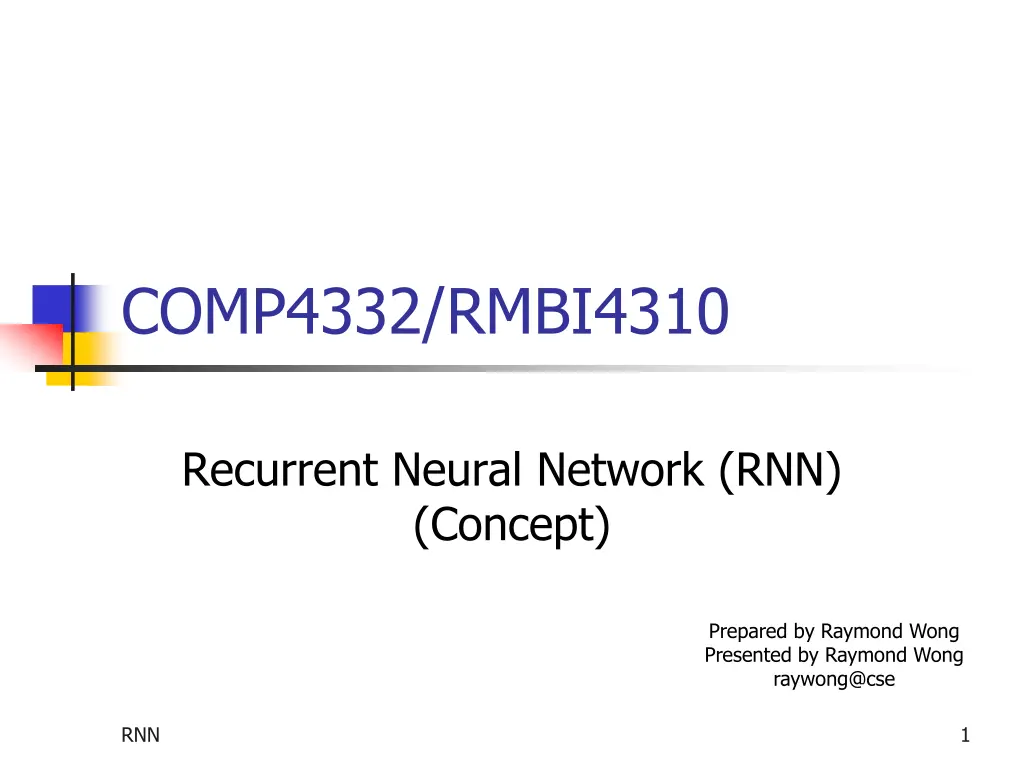
COMP4332/RMBI4310 Recurrent Neural Network (RNN) (Concept) Prepared by Raymond Wong Presented by Raymond Wong raywong@cse RNN 1

We have learnt a neural network. In this set of lecture notes, we will learn a new concept called recurrent neural network (RNN) . RNN 2

x1 0 0 1 1 x2 0 1 0 1 d 0 1 1 1 Neural Network We train the model starting from the first record. Neural Network input x1 output Neural Network y x2 Output attribute Input attributes RNN 3

x1 0 0 1 1 x2 0 1 0 1 d 0 1 1 1 Neural Network Neural Network input x1 output Neural Network y x2 Output attribute Input attributes RNN 4

x1 0 0 1 1 x2 0 1 0 1 d 0 1 1 1 Neural Network Neural Network input x1 output Neural Network y x2 Output attribute Input attributes RNN 5

x1 0 0 1 1 x2 0 1 0 1 d 0 1 1 1 Neural Network Neural Network input x1 output Neural Network y x2 Output attribute Input attributes RNN 6

x1 0 0 1 1 x2 0 1 0 1 d 0 1 1 1 Neural Network We train the model with the first record again. Neural Network input x1 output Neural Network y x2 Output attribute Input attributes RNN 7

Neural Network Here, we know that training the model with one record is independent of training the model with another record This means that we assume that records in the table are independent RNN 8

In some cases, the current record is related to the previous records in the table. Thus, records in the table are dependent . We also want to capture this dependency in the model We could use a new model called recurrent neural network for this purpose. RNN 9

Neural Network Neural Network input x1 output Neural Network y x2 Output attribute Input attributes RNN 10

Neural Network Neural Network Record 1 (vector) input x1,1 output Neural Network x1 y1 x1,2 Output attribute Input attributes RNN 11

Neural Network Neural Network input x1 output Neural Network y1 Input vector Output attribute RNN 12

Recurrent Neural Network Recurrent Neural Network (RNN) Neural Network with a Loop input x1 output Recurrent Neural Network (RNN) y1 Input vector Output attribute RNN 13

Recurrent Neural Network Recurrent Neural Network (RNN) input x1 output y1 RNN Input vector Output attribute RNN 14

Unfolded representation of RNN x1 Timestamp = 1 y1 RNN x2 y2 Timestamp = 2 RNN x3 y3 Timestamp = 3 RNN xt yt Timestamp = t RNN RNN 15

xt-1 Timestamp = t-1 yt-1 RNN Internal state variable st-1 xt yt Timestamp = t RNN Internal state variable st xt+1 yt+1 Timestamp = t+1 RNN st+1 Internal state variable RNN 16

xt-1 yt-1 Timestamp = t-1 RNN st-1 xt Timestamp = t RNN yt st xt+1 Timestamp = t+1 yt+1 RNN RNN 17

There are many applications for a recurrent neural network. Application 1 Prediction/Classification/Regression on Time series data Application 2 Translation from one language (e.g., English) to another language (e.g., French) All values recorded as a single timestamp correspond to a record in the table Each sentence in one language and the corresponding sentence in another language correspond to a record in the table. RNN 18

Application 3 Automatic Handwriting Generation Consider a letter. Each coordinate along the path/trajectory of writing this letter corresponds to a record in the table. RNN 19

Application 4 Automatic Image Caption Generation Use some existing models to generate a list of keywords for a given image. Then, use the RNN model to generate a complete sentence based on these keywords. In the RNN model, a list of consecutive words (from existing articles) corresponds to a record in the table. RNN 20

s RNN 21

Limitation It may memorize a lot of past events/values Due to its complex structure, it is more time-consuming for training. RNN 22

RNN 1. Basic RNN 2. Traditional LSTM 3. GRU RNN 23

Basic RNN The basic RNN is very simple. It contains only one single activation function (e.g., tanh and ReLU ). RNN 24

xt-1 yt-1 Timestamp = t-1 RNN st-1 xt Timestamp = t RNN yt st xt+1 Timestamp = t+1 yt+1 RNN RNN 25

xt-1 yt-1 Timestamp = t-1 Basic RNN st-1 xt Timestamp = t Basic RNN yt st xt+1 Timestamp = t+1 yt+1 Basic RNN RNN 26

xt-1 yt-1 Timestamp = t-1 Basic RNN st-1 xt Timestamp = t Memory Unit Basic RNN yt st xt+1 Timestamp = t+1 yt+1 Basic RNN RNN 27

xt-1 yt-1 Timestamp = t-1 Basic RNN st-1 Activation Function xt Timestamp = t Usually, it is tanh or ReLU yt st xt+1 Timestamp = t+1 yt+1 Basic RNN RNN 28

0.7 0.3 W = b = 0.4 xt-1 yt-1 Timestamp = t-1 Basic RNN 0.4 st-1 Activation Function xt Timestamp = t st = tanh(W . [xt, st-1] + b) st = tanh(W . [xt, st-1] + b) yt = st yt = st yt st xt+1 Timestamp = t+1 yt+1 Basic RNN RNN 29

In the following, we want to compute (weight) values in the basic RNN. Similar to the neural network, the basic RNN model has two steps. Step 1 (Input Forward Propagation) Step 2 (Error Backward Propagation) In the following, we focus on Input Forward Propagation . In the basic RNN, Error Backward Propagation could be solved by an existing optimization tool (like Neural Network ). RNN 30

Time t=1 t=2 xt, 1 0.1 0.7 xt, 2 0.4 0.9 y 0.3 0.5 Consider this example with two timestamps. When t = 1 When t = 2 We use the basic RNN to do the training. RNN 31

When t = 1 xt-1 x0 yt-1 y0 Timestamp = t-1 0 Basic RNN st-1 s0 Activation Function xt x1 1 Timestamp = t st = tanh(W . [xt, st-1] + b) st = tanh(W . [xt, st-1] + b) yt = st yt = st yt y1 s1 st xt+1 x2 2 Timestamp = t+1 yt+1 y2 Basic RNN RNN 32

st = tanh(W . [xt, st-1] + b) Time t=1 t=2 xt, 1 0.1 0.7 xt, 2 0.4 0.9 y yt = st 0.3 0.5 Step 1 (Input Forward Propagation) y0 0 s0 0 s1 = tanh(W . [x1, s0] + b) 0.7 0.3 0.4 = tanh(0.7 . 0.1 + 0.3 . 0.4 + 0.4 . 0 + 0.4) 0.1 0.4 0 = tanh( + 0.4) 0.7 0.3 0.4 W = b = 0.4 = tanh(0.59) = 0.5299 s1 = 0.5299 y1 = 0.5299 y1 = s1 = 0.5299 Error = y1 - y = 0.5299 0.3 = 0.2299 RNN 33

st = tanh(W . [xt, st-1] + b) Time t=1 t=2 xt, 1 0.1 0.7 xt, 2 0.4 0.9 y yt = st 0.3 0.5 Step 1 (Input Forward Propagation) s1 y0 0 s0 0 y1 0.5299 0.5299 0.7 0.3 0.4 W = b = 0.4 s1 = 0.5299 y1 = 0.5299 RNN 34

st = tanh(W . [xt, st-1] + b) Time t=1 t=2 xt, 1 0.1 0.7 xt, 2 0.4 0.9 y yt = st 0.3 0.5 Step 1 (Input Forward Propagation) s1 y0 0 s0 0 y1 0.5299 0.5299 s2 = tanh(W . [x2, s1] + b) 0.7 0.3 0.4 = tanh(0.7 . 0.7 + 0.3 . 0.9 + 0.4 . 0.5299 + 0.4) 0.7 0.9 = tanh( + 0.4) 0.7 0.3 0.4 W = b = 0.4 0.5299 = tanh(1.3720) = 0.8791 s2 = 0.8791 y2 = 0.8791 Error = y2 - y = 0.8791 0.5 y2 = s2 = 0.8791 = 0.3791 RNN 35

RNN 1. Basic RNN 2. Traditional LSTM 3. GRU RNN 36

Traditional LSTM Disadvantage of Basic RNN The basic RNN model is too simple . It could not simulate our human brain too much. It is not easy for the basic RNN model to converge (i.e., it may take a very long time to train the RNN model) RNN 37

Traditional LSTM Before we give the details of our brain, we want to emphasize that there is an internal state variable (i.e., variable st) to store our memory (i.e., a value) The next RNN to be described is called the LSTM (Long Short-Term Memory) model. RNN 38

Traditional LSTM It could simulate the brain process. Forget Feature It could decide to forget a portion of the internal state variable. Input Feature It could decide to input a portion of the input variable for the model It could decide the strength of the input for the model (i.e., the activation function) (called the weight of the input) RNN 39

Traditional LSTM Output Feature It could decide to output a portion of the output for the model It could decide the strength of the output for the model (i.e., the activation function) (called the weight of the output) RNN 40

Traditional LSTM Our brain includes the following steps. Forget component Input component Input activation component Internal state component Output component Final output component Forget gate Input gate Input activation gate Input state gate Output gate Final output gate RNN 41

xt-1 yt-1 Timestamp = t-1 RNN st-1 xt Timestamp = t RNN yt st xt+1 Timestamp = t+1 yt+1 RNN RNN 42

xt-1 yt-1 Timestamp = t-1 Traditional LSTM st-1 xt Timestamp = t Traditional LSTM yt st xt+1 Timestamp = t+1 yt+1 Traditional LSTM RNN 43

xt-1 yt-1 Timestamp = t-1 Traditional LSTM st-1 xt Timestamp = t Memory Unit Traditional LSTM yt st xt+1 Timestamp = t+1 yt+1 Traditional LSTM RNN 44

0.7 0.3 Wf = bf = 0.4 xt-1 yt-1 Timestamp = t-1 Traditional LSTM 0.4 st-1 ft xt Timestamp = t ft = (Wf [xt, yt-1] + bf) Forget gate ft = (Wf [xt, yt-1] + bf) Sigmoid function (net) yt 1 y = 1 + e-net st xt+1 Timestamp = t+1 yt+1 Traditional LSTM RNN 45

0.2 0.3 bi = 0.2 Wi = xt-1 yt-1 Traditional LSTM 0.4 Timestamp = t-1 st-1 ft xt Timestamp = t it ft = (Wf [xt, yt-1] + bf) it = (Wi [xt, yt-1] + bi) Input gate it = (Wi [xt, yt-1] + bi) yt st xt+1 Timestamp = t+1 yt+1 Traditional LSTM RNN 46

0.4 0.2 ba = 0.5 Wa = xt-1 yt-1 Timestamp = t-1 Traditional LSTM 0.1 st-1 ft xt Timestamp = t it ft = (Wf [xt, yt-1] + bf) it = (Wi [xt, yt-1] + bi) at tanh at = tanh(Wa [xt, yt-1] + ba) Input activation gate yt at = tanh(Wa [xt, yt-1] + ba) st tanh function tanh(net) xt+1 Timestamp = t+1 yt+1 Traditional LSTM y = e2 net 1 e2 net + 1 RNN 47

xt-1 yt-1 Timestamp = t-1 Traditional LSTM st-1 ft xt Timestamp = t it ft = (Wf [xt, yt-1] + bf) it = (Wi [xt, yt-1] + bi) at tanh at = tanh(Wa [xt, yt-1] + ba) yt st xt+1 Timestamp = t+1 yt+1 Traditional LSTM RNN 48

xt-1 yt-1 Timestamp = t-1 Traditional LSTM st-1 ft xt Timestamp = t x it ft = (Wf [xt, yt-1] + bf) it = (Wi [xt, yt-1] + bi) at + tanh x at = tanh(Wa [xt, yt-1] + ba) st = ft. st-1 + it. at Internal state gate yt st = ft. st-1 + it. at st xt+1 Timestamp = t+1 yt+1 Traditional LSTM RNN 49

xt-1 yt-1 Timestamp = t-1 Traditional LSTM st-1 ft xt Timestamp = t x it ft = (Wf [xt, yt-1] + bf) it = (Wi [xt, yt-1] + bi) at + tanh x at = tanh(Wa [xt, yt-1] + ba) st = ft. st-1 + it. at yt st xt+1 Timestamp = t+1 yt+1 Traditional LSTM RNN 50