Understanding RF Linear Accelerators Coupling Mechanisms
Explore the intricate coupling mechanisms of RF linear accelerators, including electric and magnetic coupling, resonant circuits, bandwidth considerations, impedance calculations, and coupler configurations. Delve into the detailed concepts presented by Dr. Graeme Burt from Lancaster University.

Download Presentation

Please find below an Image/Link to download the presentation.
The content on the website is provided AS IS for your information and personal use only. It may not be sold, licensed, or shared on other websites without obtaining consent from the author. If you encounter any issues during the download, it is possible that the publisher has removed the file from their server.
You are allowed to download the files provided on this website for personal or commercial use, subject to the condition that they are used lawfully. All files are the property of their respective owners.
The content on the website is provided AS IS for your information and personal use only. It may not be sold, licensed, or shared on other websites without obtaining consent from the author.
E N D
Presentation Transcript
RF Linear accelerators L3: Coupling to Standing wave cavities Dr Graeme Burt Lancaster University
Cavity Coupling Probe Loop Hook
Electric coupling use J From Gauss law = . Q E dS 0 dQ dt = I Integrated over the tip of the inner conductor. The equivalent circuit for electric coupling is a current source in parallel with a capacitance. The top rail represents the inner conductor and the ground plane is the cavity body and outer conductor. E J dV A E
Magnetic coupling use J From Faradays law dB dt = . V dS H J dV A H m The equivalent circuit for magnetic coupling where the inner conductor loops round and is connected to the outer conductor is a voltage source in series with an inductor capacitance. If the loop isn t physically connected then there is also a series capacitance making a band pass filter.
Parallel resonant circuit A resonator can be modelled as a parallel LRC circuit. Here we drive it with a current source. Applying Kirchoff s loop law gives. ( ) I t C V = + + 2 0 V V 0 Q Solving for sinusoidal varying I and V yields (Q= RC) RI e V t = + + j t 0 ( ) 0 Q 2 = tan 0 where 2 1 Q 0 0 0
Resonant Bandwidth 1.00 0.75 P 0.50 0 QL 1 tL = = 0.25 0.00 -10 -5 0 5 10 - 0 SC cavities have much smaller resonant bandwidth and longer time constants. Over the resonant bandwidth the phase of S21 also changes by 180 degrees.
Impedance and filling The cavity impedance is given as the voltage divided by the current. j V I Re = = Z c 2 + 2 1 Q 0 0 If the RF is turned off the voltage will decay exponentially as the losses are proportional to the stored energy. ( ) ( ) = + / t cos V t RI e t 0 0
Couplers However the RF source has an impedance (plus the inductance of the coupler) which isn t always matched to the cavity. This can be represented as a transformer. The RF source is represented by a ideal current source in parallel to an impedance and the coupler is represented as an n:1 turn transformer. Typically Z0 is 50 Ohms but the cavity shunt impedance, R, is ~Mohms.
I=Is/n The transformer makes the load impedance seen smaller by a factor of n2 By varying the coupling we vary n allowing us to set the load impedance. Z0n2 When on resonance the cavity impedance equals the shunt impedance (Zc=R) We can then simply model the circuit as two parallel resistors.
Power Transfer Theory Vs = Is RiRL/(Ri+RL) Is PL=Vs2 / RL (the power delivered to the load) Ri RL PL = Is2 Ri2RL/ (Ri+RL)2 PL= Is2 Ri2 / (Ri2/RL +2Rs+RL) The minimum peak power occurs when ( ( ) L i L dR R R + ) 2 2 I R R R dP = = s i i L 0 L 3 Which occurs when RL=Ri In this case the load dissipates a peak power PL=Is2Ri/4
Generator Power It makes sense that the generator power from the RF source is the maximum power that can be delivered to the cavity rather than power delivered from the current source. This occurs when 2 0 Z n R = In this case the rms power delivered, P+, is P 2 2 I R n I Z += = 0 s s 2 8 8 As the coupler (n) changes or the cavity impedance changes the power from the current source will vary but we ignore this. We only care about the power dissipated in the cavity and the generator power which is fixed as above.
Travelling waves Most circuit theory makes the assumption that the voltages do not depend on cable lengths At higher frequencies this assumption is no longer true and waves propagate along the cables. Waves can propagate forwards, V+, or backwards, V-, The voltage at any point is a superposition of both waves V=V++V- The same happens with current where I=I+-I- The generator is a source of forward current, I+, not current, I, hence why we only took part of the power produced earlier. V+ V-
External Q factor Ohmic losses are not the only loss mechanism in cavities. We also have to consider the loss from the couplers. We define this external Q as, P P Q Q R U P = = = = = 2 0 e Q n Z C 0 e 2 n Z 0 c e e Where Pe is the power lost through the coupler when the RF sources are turned off. We can then define a loaded Q factor, QL, which is the real Q of the cavity Q Q Q Q 1 1 1 = 1 1 + = + 0 0 = + Q Q Q L e 0 L e U = Q L P tot
Cavity Voltage The generator power is given by: Where I use the circuit definition of R. Rearranging this gives the current The voltage is given by Hence 2 2 I Z I R = = 0 P + 8 8 2 P R = + 2 I 2 IRZ n R + IR + = = = 0 V IR c tot 2 1 n Z 0 2 2 RP + + = V c 1
Reflected Power Z Z 2 2 2 I Z 4 I Z Z = s 0 s 0 c P The reflected power in steady state operation is the power supplied to the cavity minus the power that is dissipated in the cavity. Here we assume a matched system and look at the power dissipated in the cavity resistance by looking at the power lost in two parallel resistors. ( ) R 2 + 0 c 2 I Z 4 4Z Z Z Z = 1 s 0 0 c P ( ) R 2 + 0 c ( ( ) ) 2 + + Z Z 4Z Z Z Z = 0 c 0 c P P ( ) R g 2 2 + Z Z 0 0 c c + + 2 2 2 + 4Z Z Z Z Z Z Z Is = 0 0 0 c c c P P ( ) R g 2 Z 0 c Ri RL ( ( ) ) 2 + Z Z = 0 c P P R g 2 Z Z 0 c
Scattering Parameters When making RF measurements, the most common measurement is the S- parameters. Input signal Black Box S2,1 S1,1 forward transmission coefficient input reflection coefficient The S matrix is a m-by-m matrix (where m is the number of available measurement ports). The elements are labelled S parameters of form Sab where a is the measurement port and b is the input port. S11 S12 S = S21 S22 The meaning of an S parameter is the ratio of the voltage measured at the measurement port to the voltage at the input port (assuming a CW input). Sab =Va / Vb
Reflected Voltage ) ) c Z + + Q ( ( 2 + Z Z = 0 c P P R g 2 Z 0 2 1 1 i i = P P R g = 0 where 0 S11 1.00 + + 1 1 i i = = 0.75 V P V + R 0.50 + + 1 1 V V i i 0.25 = = S 11 0.00 + -10 -5 0 5 10 f
Polar plot of S11 Plotting the Re and imaginary components give a polar plot. + + 1 1 i i = = V P V + R + + 1 1 V V i i = = S 11 +
Under and Over coupled Beta=Q0/Qe < 1 Beta = 1 Beta > 1 We can tell if beta is greater or less than 1 from the polar plot. If the circle doesn t circle the origin then beta is less than 1 (undercoupled) If the circle does circle the origin then beta is greater than 1 (overcoupled)
Cavity Coupling Cavity Behaviour examples Steady state The most important behaviour we must understand is when the cavity is in steady state (ie when the cavity stored energy is constant and U=U0). We can use the definitions of beta and Q to derive, 4 + P Q f = 0 U ( ) 0 2 1 We can also get voltage by using R/Q (remember the overvoltage). From this equation we can see that the cavity energy is maximum when =1 (also when the reflections are zero and all power is dissipated in the cavity) 2 1 = P P r f + 1
Filling time The cavity fills with time as 1-e-t/ where t is the filling constant/time. 2 2 RP + ( ) + = / t 1 V e c 1 The filling constant is =2QL/ The higher the loaded Q the higher the stored energy but the longer it takes to fill.
Transient reflections The reflections are also not constant. They actually vary with time. When we first apply a pulse all the wave is reflected, but as the cavity fills its emitted power cancels the reflected signal. ) 0.8 for P + 2 2 RP + = V c 1 As we know the voltage increases as 1-e-t/ with time 2 2 RP + ( 1 P + = / t 1 V e ref = 0.1 c 1 Using the definition of reflected voltage and knowing that V+ is constant 0.6 = 1 = 10 0.4 = V V V + 0.2 2 1 ( ) = / t 1 1 V V e 0 + + 0 1 2 3 4 5 0/2 t Q L
Cavity Filling When filling, the impedance of a resonant cavity varies with time and hence so does the match this means the reflections vary as the cavity fills. note: No beam! 1 P P ref = 0.1 0.8 for 0.6 As we vary the external Q of a cavity the filling behaves differently. Initially all power is reflected from the cavity, as the cavities fill the reflections reduce. = 1 = 10 0.4 0.2 0 0 1 2 3 4 5 0/2 t Q L The cavity is only matched (reflections=0) if the external Q of the cavity is equal to the ohmic Q (you may include beam losses in this). A conceptual explanation for this as the reflected power from the coupler and the emitted power from the cavity destructively interfere.
Coupling Strength Excited by a square pulse critically coupled under coupled over coupled 2 2 2 = = 2 = 1 0.5 1.5 1.5 1.5 P P ref 1 1 1 for 0.5 0.5 0.5 0 0 0 0 2 4 6 8 10 0 2 4 6 8 10 0 2 4 6 0/2 t 8 10 Q L
Excitation of the CI compact linac 0.0 9.24 9.26 9.28 9.3 9.32 9.34 9.36 -5.0 -10.0 -15.0 S11, dB -20.0 -25.0 -30.0 -35.0 -40.0 Freq, GHz water OFF T=19 deg 20 22 25 LHS shows the filling of the cavity off tune.
Microphonics Microphonics cause the cavity resonant frequency to oscillate in time. As we have seen before the reflections are dependant on the difference between the drive and natural frequencies. + + 1 1 i i = = V P V + R + + 1 1 V V i i = = S 11 + As the detuning angle is proportional to the Q factor it leads to an optimal coupling for SRF cavities, which have high Q s. This has been an issue in the DICC. S11 1.00 0.75 0.50 0.25 0.00 -10 -5 0 5 10 f
Microphonics As can be seen if the microphonics cause a detuning larger than the cavity bandwidth the power demand to keep the cavity at the required voltage is large. To avoid this a lower external Q is chosen than the ohmic Q, ie the coupler is not matched. This leads to higher reflections without microphonics but much lower reflections in practice ( 8 ) 2 + 2 1 R V 2 = 1 4 + c 2 P Q + L 2 1000 No microphonics 800 power required 100 Hz 600 200 Hz 400 400 Hz 200 0 1.E+06 1.E+07 External Q 1.E+08 Power demand for 1 watt ohmic heating in ALICE
Beam Loading In addition to ohmic losses we must also consider the power extracted from the cavity by the beam. The beam draws a power Pb=Vc Ibeam from the cavity. Ibeam=q f, where q is the bunch charge and f is the repetition rate This acts as a current source in series with the cavity I=Is/n Ib Z0n2
Coupling with Beam Loading The rf source will not see any difference between the power dissipated in the cavity walls and the power extracted by the beam hence we can calculate a new Q factor, Qcb. U + = Q cb P P c b this Qcb will replace Q0 when calculating cavity filling. This means the match will change as well as needing more power. + Q Q 4 P Q = cb eb f = cb U eb ( ) 0 2 1 e eb Normally we aim for =1 with beam and have reflections when filling. Q Q Pb Pc = = + 1 0 e
Detuning In many RF systems the beam is not accelerated on crest, but at a phase slightly above or below the maximum voltage. In this case the beam induces a current in the cavity which is out of phase with the main RF and hence changes the cavity phase Beam V 2.5 2 1.5 1 0.5 0 0 1 2 3 4 5 6 -0.5 V before beam arrives -1 -1.5 -2 -2.5 This causes a phase (and frequency) shift as the imaginary part remains the same. Phase shift = atan [(Ib R/Q)/Vg]
Solution to detuning The phase/frequency shift is effectively adding a capacitance to the cavity circuit. This can be fixed by detuning the cavity so that we reduce the cavities capacitance accordingly. Lets assume the case of a bunch in quadrature with the RF system. The cavity phase is advanced between bunches because it is at a higher frequency (real part becomes finite and negative). The beam causes a phase (and frequency) shift as the imaginary part remains the same. Phase shift = atan [(Ib R/Q)/Vg] The two phase shifts cancel if I R V Q b 0 2 g If correct cavity frequency is chosen beam loading is reduced as the real parts cancel. However imaginary part also changes. However without beam the cavity has the wrong frequency.
Required Power with beam In this case the power is ( ) 2 + + 1 P P c b = P g 4 P c Where 1 2 R Q sin P I V q b b g s Normally the 2nd term on the RHS is neglected. In an ERL the loading due to the injected and spent beam exactly cancel. This means that the beamloading can be neglected
Beamloading (no microphonics) 1000 900 No beam 800 700 100 uA power required 600 200 uA 500 400 400 uA 300 200 100 0 1.E+06 1.E+07 External Q 1.E+08
Beamloading (200 Hz microphonics) 1000 900 No beam 800 700 100 uA power required 600 200 uA 500 400 400 uA 300 200 100 0 1.E+06 1.E+07 External Q 1.E+08
SRF Couplers Also a limited power in SRF couplers. WG limited to 500 kW due to multipactor (electron cloud). Coax is limited to a similar amount by limited cooling of inner coax.


")
")