Explore the familiar concept of probability in healthcare, where chances of outcomes are vital in decision-making. Learn about classical and relative frequency probabilities, and how they apply to medical scenarios, providing a foundation for informed assessments and care.
Please find below an Image/Link to download the presentation.
The content on the website is provided AS IS for your information and personal use only. It may not be sold, licensed, or shared on other websites without obtaining consent from the author. If you encounter any issues during the download, it is possible that the publisher has removed the file from their server.
You are allowed to download the files provided on this website for personal or commercial use, subject to the condition that they are used lawfully. All files are the property of their respective owners.
The content on the website is provided AS IS for your information and personal use only. It may not be sold, licensed, or shared on other websites without obtaining consent from the author.
E N D
Presentation Transcript
The concept of probability is not a foreign to health workers and is frequently encountered in everyday activities, it is a familial concept as example when we hear a physician giving the chance of surviving from certain operation to a patient such as 50 - 50 chance of surviving (meaning 50% to survive and 50% chances to death out of 100%). Thus we are accustomed to measure the probability of the occurrence of some event by a number between zero and one. The more likely the event, the closer the number is to one; and the more unlikely the event, the closer the number is to zero.
An event that cannot occur has a probability of zero, An event that less likely to occur has a probability near to zero, An event that is certain to occur has a probability of one, and An event that is most likely to occur has a probability near to one.
The concept of objective probability that is derived from objective processes is of two types: 1- Classical probability (Priori Probability): Developed out of the attempts to solve problems related to games of chance. For example; Coin: the rolling of coin will give only two results (Head, Tail) with equally likely chances of each one to occur and that there is no reason to favour the drawing of anyone. P H= 1/2= 0.5 P T= 1/2= 0.5 Total P.= 1
Dice: the rolling of dice will give only 6 results (1,2,3,4,5 & 6) with probability of 1/6 for the appearance of any number and the total probability of 1. Cards: we have 52 cards (of two colors red and black, of 4 types) so probability of selecting of one card is 1/52. The probability here depend on whether the events are mutually exclusive or not (the two events does not occur at the same time). The probability is calculated by the process of abstract reasoning. It is calculated by many methods; addition, multiplication, factorial, or combination.
2- Relative frequency probability (Posteriori Probability): It depends on the repeatability of some process and the ability to count the number of repetitions, as well as the number of times that some event of interest occurs.
From this data that show the probability distribution of this continuous random variable (and even for the discrete type), it is clear that the column of relative frequency, it show corresponding positive values, they are all less than 1, and their sum is equal to 1. These are the characteristics of probability distribution, which also represent the relative frequency of occurrence of such values, also we can obtain the cumulative probability by adding the probability through the relative frequency from cumulating it, and it gives a good determination of probability.
There are different theoretical types of probability distribution; 1- Binomial Prob. Distribution. 2- Poisson Prob. Distribution. 3- Normal Prob. Distribution. 4- Skewed Prob. Distribution.
The line when deal with probability distribution has some characteristics; - Smooth curve - Total area under the curve is equal to one. - Relative frequency (f/n) of occurrence of value between any two points on x-axis is equal to the area bounded by the curve and the two points.
Normal distribution curve: The graph of normal distribution produces the bell- shaped curve. It is the most important type of distribution in all of statistics. It is also called Gaussian distribution. It has the following characteristics; 1- It is symmetrical about its mean. 2- The mean, mode and median are equal. 3- The total area under the curve above the x-axis is one unit. 4- The normal distribution curve is completely determined by two parameters (mean & standard deviation). 5- 68% of the total area under the curve is enclosed by mean +1 SD, 95% of the total area is enclosed by mean + 2 SD & 99.7% enclosed under mean + 3 SD.
The importance of normal distribution: 1. It is a good empirical description of many variables and especially the biological variables of human being, all laboratory investigations and body measurements. 2. It represents the bases of statistical analysis and testing hypothesis, so any data to be tested should be normally distributed or assumed to be normally distributed.
Sampling variation & Standard error: The sample mean is unlikely to be exactly equal to the population mean ( ) (mu) as a different sample would give a different estimate, the difference being due to sampling variation. If we collect many independent samples of the same size and calculate the sample mean of each of them, then a frequency distribution of those means could be formed. The mean of this distribution would be the population mean ( ), and it can be shown that its standard deviation would be equal to SD / n .
This is called the standard error of the sample mean and it measures how precisely the population mean is estimated by sample mean. Sampling variation; is the degree of variability of sample mean from the population mean from which we the sample were taken. SE; is the measurement of the degree of variability of sample mean from population mean from which the sample were taken.
The size of SE depends on: 1- Variation in the population (SD,..) 2- Size of the sample (n). We use sample SD to estimate the SE by: