Understanding Wigner Distribution Function for Time-Frequency Analysis
Explore the Wigner Distribution Function (WDF) and its significance in joint time-frequency analysis, along with related operators and computations in the frequency domain. Discover why the WDF offers higher clarity compared to other methods and its role in signal analysis. Delve into key references and concepts shaping time-frequency signal analysis.

Download Presentation

Please find below an Image/Link to download the presentation.
The content on the website is provided AS IS for your information and personal use only. It may not be sold, licensed, or shared on other websites without obtaining consent from the author. If you encounter any issues during the download, it is possible that the publisher has removed the file from their server.
You are allowed to download the files provided on this website for personal or commercial use, subject to the condition that they are used lawfully. All files are the property of their respective owners.
The content on the website is provided AS IS for your information and personal use only. It may not be sold, licensed, or shared on other websites without obtaining consent from the author.
E N D
Presentation Transcript
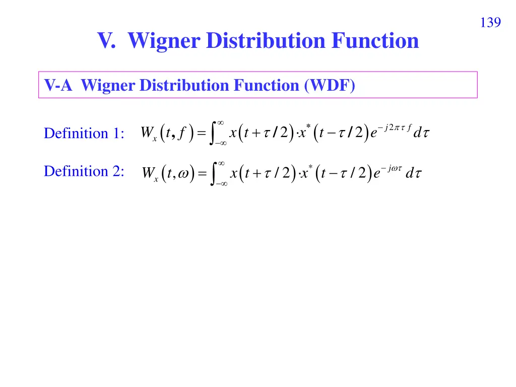
139 V. Wigner Distribution Function V-A Wigner Distribution Function (WDF) ( ) ( ) ( ) = + x t * 2 j f , / / 2 2 W t f x t e d Definition 1: x ( ) ( ) ( ) Definition 2: = + x t * j , / 2 / 2 W t x t e d x
140 Another way for computation from the frequency domain ( ) ( ) ( ) = + X * 2 j t , / / 2 2 W t f X f f e d Definition 1: x where X(f) is the Fourier transform of x(t) ( ) ( ) ( ) j t , = + X * / / Definition 2: 2 2 W t X e d x The Wigner distribution function is also called the Wigner Ville distribution.
141 Main Reference [Ref] S. Qian and D. Chen, Joint Time-Frequency Analysis: Methods and Applications, Chap. 5, Prentice Hall, N.J., 1996. Other References [Ref] E. P. Wigner, On the quantum correlation for thermodynamic equilibrium, Phys. Rev., vol. 40, pp. 749-759, 1932. [Ref] T. A. C. M. Classen and W. F. G. Mecklenbrauker, The Wigner distribution A tool for time-frequency signal analysis; Part I, Philips J. Res., vol. 35, pp. 217-250, 1980. [Ref] F. Hlawatsch and G. F. Boudreaux Bartels, quadratic time-frequency signal representation, IEEE Signal Processing Magazine, pp. 21-67,Apr. 1992. [Ref] R. L. Allen and D. W. Mills, Signal Analysis: Time, Frequency, Scale, and Structure, Wiley-Interscience, NJ, 2004. Linear and
142 The operators that are related to the WDF: (a) Signal auto-correlation function: ( ) ( , x C t x t = ) ( ) + /2 /2 x t (b) Spectrum auto-correlation function: ( ) ( , f X f = ) ( ) + /2 /2 xS X f (c) Ambiguity function (AF): ( ) , = ( ) ( ) + * 2 j t / 2 / 2 x A x t x t e x(t) dt FT f FTt Cx(t, ) FT f IFT t Ax( , ) Wx(t, f ) X(f) Sx( , f ) IFT t IFTf
143 V-B Why the WDF Has Higher Clarity? Due to signal auto-correlation function f (1) If x(t) = 1 (2) If x(t) = exp(j2 h t) t ( ) + = 2 ( /2) 2 ( /2) 2 j h t j h t j f , W t f e e e d x f = 2 2 j h j f e e d f h = 2 ( ) j e d t = ( ) f h Comparing: for the case of the STFT
144 f (3) If x(t) = exp(j2 k t2) t (4) If x(t) = (t) f ( ) ( ) ( ) = + 2 j f , / / 2 2 W t f t t e d x ( ) ( ) Page 138 (2) = + 2 j f 4 2 2 t t e d t ( ) 4 Page 138 (4) ( ) t e ( ) t = = = 4 4 j t f j t f 4 t e ( ) ( ) y d Page 138 (2) Page 138 (5), t0= 0 0 ( ) = y 0
145 V-C The WDF is not a Linear Distribution ( ) ( ) ( ) = + x t * 2 j f , /2 /2 W t f x t e d x If h(t) = g(t) + s(t) ( ) ( ) ( ) = + h t * 2 j f , /2 /2 W t f h t e d h ( ) ( ) ( ) ( ) = + + + + 2 j f /2 /2 /2 /2 g t s t g t s t e d ( ) ( ) ( ) ( s t ) = + + + 2 2 | | /2 /2 | | /2 /2 g t g t s t ( ) ( s t ) ( ) ( s t ) + + ) ) /2 + + 2 j f /2 /2 ( /2 /2 g t g t e d ( ) = + 2 2 | | , | | , W t f W t f g s ( ) ( s t ( ) ( s t ) + + + + 2 j f /2 /2 /2 g t g t e d cross terms
146 V-D Examples of the WDF Simulations x(t) = cos(2 t) = 0.5[exp(j2 t) + exp(-j2 t)] by the WDF by the Gabor transform -5 5 f-axis f-axis f-axis f-axis 1 1 0 0 -1 -1 5 -5 0 2 4 6 8 10 0 2 4 6 8 10 t-axis t-axis t-axis t-axis
147 ( ) x t : rectangular function = (( 5)/4) t by the WDF by the Gabor transform -5 -5 -4 f-axis f-axis -3 f-axis f-axis -2 -1 0 0 1 2 3 4 5 0 2 4 6 8 10 0 2 4 6 8 10 t-axis t-axis t-axis t-axis
148 ( ) x t = 2 exp ( 5) t by the WDF by the Gabor transform 5 -5 -4 f-axis f-axis f-axis f-axis -3 -2 -1 0 0 1 2 3 4 -5 0 2 4 6 8 10 0 2 4 6 8 10 t-axis t-axis t-axis t-axis 2 2 FT t f e e Gaussian function: Gaussian function s T-F area is minimal.
149 ( ( ) ( ) s t = 2 for 9 t 1, s(t) = 0 otherwise, exp /10 3 jt j t ) ( ) r t = + 2 2 exp /2 6 exp j t ( 4) /10 jt t f (t) = s(t) + r(t) : t-axis, : f -axis
150 ( ) x t = 3 exp( ( 5) 6 ) j t j t by the WDF by the Gabor transform 5 4 f-axis f-axis 3 f-axis f-axis 2 1 0 0 -1 -2 -3 -4 -5 -5 0 2 4 6 8 10 0 2 4 6 8 10 t-axis t-axis t-axis t-axis
151 V-E Digital Implementation of the WDF ( ) ( ) ( ) , = + x t * 2 j f , /2 /2 W t f x t e d x ( ) ( ) ( ) (using = /2 ) = + x t * 4 j f , 2 W t f x t e d x Sampling: t = n t, f = m f, = p t ( ) ( ) ( ) ( ) = + , 2 ( ) ( ) exp 4 W n m x n p x n p j mp x t f t t t f t = p When x(t) is not a time-limited signal, it is hard to implement.
152 Suppose that x(t) = 0 for t < n1 tand t > n2 t x(t) n1 t n t n2 t ( ) ( ) + only when n + p [n1, n2] and n p [n1, n2] ( ) ( ) 0 x n p x n p t t p ( n ) n1 n + p n2 n1 n p n2 n1 n p n2 n n1 n p n2 n, n n2 p n n1 max(n1 n , n n2) p min(n2 n , n n1) min(n2 n , n n1) p min(n2 n , n n1)
153 x(t) n1 t n t n2 t (n n1) t (n2 n) t min(n2 n , n n1) p min(n2 n , n n1) Q Q = min(n2 n, n n1). Q (n2 n) t, (n n1 ) t: n > n2 Q < 0 p n < n1 ( ) = , 0 W n m x t f
154 If x(t) = 0 for t < n1 tand t > n2 t Q ( ) ( ) ( ) ( ) = + , 2 ( ) ( ) exp 4 W n m x n p x n p j mp x t f t t t f t T F = p Q Q = min(n2 n, n n1). (varies with n) p [ Q, Q], n [n1, n2], possible for implementation Method 1: Direct Implementation (brute force method)
155 3 Method 2: Using the DFT 1 When and N 2Max(Q)+1 = 2(n2-n1)/2+1 = n2-n1+1 = T 2 N ( , 2 ( ) x t f t p Q = T F = t f Q ) 2 mp N ( ) ( ) j = + ( ) W n m x n p x n p e t t q = p+Q p = q Q 2 Q ( ) 2 2 mQ N mq N ( ) ( ) j j = q Q + n q Q + , 2 ( ) ( ) W n m e x n x e x t f t t t = 0 q 1 N Q = min(n2 n, n n1). n [n1, n2], ( ) 2 2 mQ N mq N ( ) j j = , 2 W n m e c q e 1 x t f t = 0 q ( = ) ) ( ( ) ( ) ( = q Q + ( ( x n n q Q + ( ) ( ) c q x n ) k x for 0 q 2Q for -Q k Q (k = q-Q) 1 t t ) i.e., + + ) ( ) c Q k x n k 1 t t ( ) c q = 0 for 2Q+1 q N 1 1
156 t = n0 t, (n0+1) t, (n0+2) t, , n1 t f = m0 f, (m0+1) f, (m0+2) f, , m1 f Step 1: Calculate n0, n1, m0, m1, N Step 2: n = n0 Step 3: Determine Q Step 4: Determine c1(q) Step 5: C1(m) = FFT[c1(q)] Step 6: Convert C1(m) into C( n t, m f) Step 7: Set n = n+1 and return to Step 3 until n = n1.
157 Method 3: Using the Chirp Z Transform Q ( ) ( ) ( ) ( ) = + , 2 ( ) ( ) exp 4 W n m x n p x n p j mp x t f t t t f t = p Q Q ( ) ( ) ( ) 2 2 2 2 ( p m 2 2 ) j m j p j = + , 2 ( ) ( ) W n m e x n p x n p e e t f t f t f x t f t t t = p Q ( ) ( ) ( ) 2 2 j p = + , ( ) ( ) x n p x n p x n p e t f Step 1 1 t t Q c m 2 2 j m = = e , , X n m x n p c m p t f Step 2 2 1 = p Q ) ( 2 2 j m = , 2 , X n m e X n m t f Step 3 2 t f t
158 Q What is the complexity of Method 1? Q What is the complexity of Method 2? Q What is the complexity of Method 3? The computation time of the WDF is more than those of the rec-STFT and the Gabor transform.
159 V-F Properties of the WDF (1) Projection property ( ) x t ( ) ( ) ( ) 2 2 = = , , W t f df X f W t f dt x x (2) Energy preservation property (3) Recovery property ( ) ( ) x t ( ) 2 2 = = , W t f dtdf dt X f df x ( ( ( ) x t ) ) ( ) x t ( ) x t ( ) 0 x*(0) = 2 j f t / 2, W t f e df x x ( ) ( ) 0 = 2 j f t , /2 W t f e dt X f X x ( ) ( ( x ( ) ( ) t ( ) f (4) Mean condition frequency and mean condition time 2 2 j j = ( ) x t = ) e X f X f e If , then ( ) t = ( ) f 2 f W t f , df x 2 ( ) ) = t W t f , X f dt ( ) 2 = n n , ( ) (5) Moment properties , t W t f dtdf t x t dt x ( ) 2 = n n , ( ) f W t f dtdf f X f df x
160 (6) Wx(t, f ) is bound to be real ( , ) = W t f ( , ) W t f x x (7) Region properties If x(t) = 0 for t > t2 then Wx(t, f ) = 0 for t > t2 If x(t) = 0 for t < t1 then Wx(t, f ) = 0 for t < t1 If , then ( ) ( ) ( ) y t x t h t = ( ) ( ) , , y x W t f W t W t f ( ) ( ) ( ) y t x t h ( ) ( ) , , y x W t f W f ( ) ( , , y x W t f W (8) Multiplication theory ( ) = , d h = (9) Convolution theory If , then ( d ) = , W t f d h ( ) ( ) ( ) ) f (10) Correlation theory If , then = + y t x t h d = ( ) + , W t f d h
161 ( ) ( ) ( = y t x t ) = t (11) Time-shifting property If , then 0 ( ) , , W t f W t t f 0 y x ) ( ) f t x t ( , W t f ( ( ) t ( y (12) Modulation property If , then = exp ) 2 y j 0 ) = , W t f f 0 x ( ) ( ) = ) (13) Constant multiplication property If , then ( x y t ( ( ) y t W t f ( ) y t ( , y cx t ) 2 = , , W t f c W t f y ( ) = (14) Conjugation property If , then ( , x W t ( ) x ct 1 | | c = , x t ) ( ) f y = ) (15) Scaling property If W t f , then ( ) 1 c = , W ct f x The STFT (including the rec-STFT, the Gabor transform) does not have real region, multiplication, convolution, and correlation properties.
162 Why the WDF is always real? What are the advantages and disadvantages it causes? Try to prove of the projection and recovery properties
163 ( ) ( ) ( ) = + x t * 2 j f , /2 /2 W t f x t e d x Proof of the region properties If x(t) = 0 for t < t0, x(t + /2) = 0 for < (t0 t)/2 = (t t0)/2, x(t /2) = 0 for > (t t0)/2, Therefore, if t t0< 0, the nonzero regions of x(t + /2) and x(t /2) does not overlap and x(t + /2) x*(t /2) = 0 for all . The importance of the region property
164 Extra Property: (16) The relation between the WDF and the spectrogram: Suppose that x(t) is the input function, w(t) is the window function of the STFT, X(t, f) is the STFT of x(t), and Wx(t, f) and Ww(t, f) are the WDFs of x(t) and w(t), respectively, then ( ) ( ) ( ) ( ) ( ) 2 = = , , , , , X t f W t f W t f W t u f v W u v dudv x w x w ( ) ( ) (Proof): , , W t u f v W u v dudv x w ( ) ( ) 2 ( f v = + ) j / 2 / 2 x t u x t u e d + d dudv 2 j v w u w u e 2 2 ) ( ) ( = + + 2 j f x t u x t u w u w u e 2 2 2 2 ( ) 2 j v dvd d du e (Cont.)
165 ) ( ) ( = + + 2 j f x t u x t u w u w u e 2 2 2 2 ( ) d d du ) ( ) ( ) ( ) ( = + + d du 2 j f x t u x t u w u w u e 2 2 2 2 = + = , t u t u Set 1 2 2 2 / / / / u u 1 1 d d = d du = d du det 1 2 2 2 ( ) ( ) ( 2 ) ( w t ) = d d 2 ( ) j f x x w t e 1 2 1 2 1 1 2 ( ) ( ) ) , ) ( ) ( 2 ) = 2 2 j f j f x w t e d x w t e d 1 2 1 1 1 2 2 ( ( ( ) = , , X t f X t f 2 = X t f
166 V-G Advantages and Disadvantages of the WDF Advantages: clarity many good properties suitable for analyzing the random process Disadvantages: cross-term problem ( ) n n exp , 0,1,2 jt not suitable for more time for computation, especial for the signal with long time duration not one-to-one
167 V-H Windowed Wigner Distribution Function When x(t) is not time-limited, its WDF is hard for implementation ( ) ( ) ( ) = + x t * 2 j f , /2 /2 W t f x t e d x with mask ( ) ( ) ( ) ( ) = + x t * 2 j f , /2 /2 W t f w x t e d x w( ) is real and time-limited The windowed WDF is also called the pseudo Wigner-Ville distribution. Advantages: (1) reduce the computation time (2) may reduce the cross term problem Disadvantages:
168 ( ) ( ) ( x t ) ( ) = + x t * 4 j f , 2 2 W t f w e d x ( ) ( ) ( x n ) ( ) 4 j mp = + , 2 2 ( ) ( ) W n m w p p x n p e t f x t f t t t t = p Suppose that w(t) = 0 for |t| > B ( ) for p < Q and p > Q B Q = p = 2 0 w t 2 t Q ( ) ( ) ( x n ) ( ) 4 j mp = + , 2 2 ( ) ( ) W n m w p p x n p e t f x t f t t t t = p Q mask
169 (B) Why the cross term problem can be avoided ? ( ) ( ) ( ) ( ) = + x t * 2 j f , /2 /2 W t f w x t e d x w( ) is real Viewing the case where x(t) = (t t1) + (t t2) x(t) t-axis t1 t2
170 ( ) W t f = , 0 for t t1, t2 ( mask function) x mask function w( ) = 1 x(t) = (t t1) + (t t2) ( ) ( ( ) ( ) = + 2 j f , / 2 / 2 W t f x t x t e d x ) ) ) ) ( ( ( = + + + + 2 j f t t t t t t t t e d 1 2 1 2 2 from page 138, property 2 2 2 2 ( ) ( ) ( ) ( ) = + + + + + + 2 j f 4 2 2 2 2 2 2 2 2 t t t t t t t t e d 1 2 1 2 ) 1 2 t ( ( ) + + + 2 2 2 t t t 2 -axis 2t1 2t 2t2 2t ) 1 2 t + ( ( ) + + 2 2 2 t t t 2 -axis 2t 2t1 2t 2t2
( + 171 ( ) 3 W t f , 0 ( ) ) + + 2 2 2 2 t t t t 1 2 x ( + ( ) ) + + 2 2 2 2 t t t t 1 2 (1) If t = t1 -axis 0 2t2 2t1 -axis 2t1 2t2 0 (2) If t = t2 -axis 2t1 2t2 0 -axis 0 2t2 2t1 (3) If t = (t1+ t2)/2 -axis t2 t1 t1 t2 -axis t2 t1 t1 t2
172 With mask function ( ) ( ) ( ) ( ) = + 2 j f , /2 /2 W t f w x t x t e d x ( ) ( ) ( ) = + + + 2 2 2 2 w t t t t 1 2 ( ) ( ) + + + 2 j f 2 2 2 2 t t t t e d 1 2 Suppose that w( ) = 0 for | | > B, B is positive. If B < t2 t1
173 B B (1) t = t1 -axis 0 2t2 2t1 -axis 2t1 2t2 (2) t = t2 -axis 2t1 2t2 0 -axis 0 2t2 2t1 -axis (3) t = (t1+ t2)/2 t1 t2 t2 t1 -axis t1 t2 t2 t1 B B
174 (1) Concepts: (2) Comparison: (3) Advantages: (3-1) Why? (4) Disadvantages: (4-1) Why? (5) Applications: (6) Innovations:
175 (1)-(5) (3-1), (4-1), (6) 100


