Unit 2- Dictation: Explore the Natural World
Embark on a journey through various landscapes and climates as you delve into the wonders of nature, from majestic continents to serene oceans and vibrant coral reefs. Discover the beauty of lush forests, towering waterfalls, and vast deserts. Experience the power of storms and thunder, the stillness of frozen landscapes, and the delicate balance of plant life. Learn about diverse ecosystems, extreme temperatures, and the dynamic forces shaping our planet. Let the images transport you to different corners of the world, inviting you to marvel at the Earth's breathtaking diversity.

Download Presentation

Please find below an Image/Link to download the presentation.
The content on the website is provided AS IS for your information and personal use only. It may not be sold, licensed, or shared on other websites without obtaining consent from the author.If you encounter any issues during the download, it is possible that the publisher has removed the file from their server.
You are allowed to download the files provided on this website for personal or commercial use, subject to the condition that they are used lawfully. All files are the property of their respective owners.
The content on the website is provided AS IS for your information and personal use only. It may not be sold, licensed, or shared on other websites without obtaining consent from the author.
E N D
Presentation Transcript
CS 5600 Computer Systems Lecture 6: Process Scheduling
Scheduling Basics Simple Schedulers Priority Schedulers Fair Share Schedulers Multi-CPU Scheduling Case Study: The Linux Kernel 2
Setting the Stage Suppose we have: A computer with N CPUs P process/threads that are ready to run Questions we need to address: In what order should the processes be run? On what CPU should each process run? 3
Factors Influencing Scheduling Characteristics of the processes Are they I/O bound or CPU bound? Do we have metadata about the processes? Example: deadlines Is their behavior predictable? Characteristics of the machine How many CPUs? Can we preempt processes? How is memory shared by the CPUs? Characteristics of the user Are the processes interactive (e.g. desktop apps) Or are the processes background jobs? 4
Basic Scheduler Architecture Scheduler selects from the ready processes, and assigns them to a CPU System may have >1 CPU Various different approaches for selecting processes Scheduling decisions are made when a process: 1. Switches from running to waiting 2. Terminates 3. Switches from running to ready 4. Switches from waiting to ready Scheduler may have access to additional information Process deadlines, data in shared memory, etc. No preemption Preemption 5
Dispatch Latency The dispatcher gives control of the CPU to the process selected by the scheduler Switches context Switching to/from kernel mode/user mode Saving the old EIP, loading the new EIP Warning: dispatching incurs a cost Context switching and mode switch are expensive Adds latency to processing times It is advantageous to minimize process switching 6
A Note on Processes & Threads Let s assume that processes and threads are equivalent for scheduling purposes Kernel supports threads System-contention scope (SCS) Each process has >=1 thread If kernel does not support threads Each process handles it s own thread scheduling Process contention scope (PCS) 7
Basic Process Behavior Processes alternate between doing work and waiting Work CPU Burst Process behavior varies I/O bound CPU bound Expected CPU burst distribution is important for scheduler design Do you expect more CPU or I/O bound processes? Process 2 Process 1 CPU Burst Execute Code Waiting on I/O Wait Execute Code Execute Code Waiting on I/O Execute Code sleep(1) Waiting for mutex Waiting on I/O Execute Code 8
Scheduling Optimization Criteria Max CPU utilization keep the CPU as busy as possible Max throughput # of processes that finish over time Min turnaround time amount of time to finish a process Min waiting time amount of time a ready process has been waiting to execute Min response time amount time between submitting a request and receiving a response E.g. time between clicking a button and seeing a response Fairness all processes receive min/max fair CPU resources No scheduler can meet all these criteria Which criteria are most important depend on types of processes and expectations of the system E.g. response time is key on the desktop Throughput is more important for MapReduce 9
Scheduling Basics Simple Schedulers Priority Schedulers Fair Share Schedulers Multi-CPU Scheduling Case Study: The Linux Kernel 10
First Come, First Serve (FCFS) Simple scheduler Processes stored in a FIFO queue Served in order of arrival Process Burst Arrival Time Time P1 24 0.000 P1 P2 P3 P2 3 0.001 Time: 0 24 27 30 P3 3 0.002 Turnaround time = completion time - arrival time P1 = 24; P2 = 27; P3 = 30 Average turnaround time: (0 + 24 + 27) / 3 = 27 11
The Convoy Effect FCFS scheduler, but the arrival order has changed Process Burst Arrival Time Time P2 P3 P1 P1 24 0.002 Time: 0 3 6 30 P2 3 0.000 P3 3 0.001 Turnaround time: P1 = 30; P2 =3; P3 = 6 Average turnaround time: (30 + 3 + 6) / 3 = 13 Much better than the previous arrival order! Convoy effect (a.k.a. head-of-line blocking) Long process can impede short processes E.g.: CPU bound process followed by I/O bound process 12
Shortest Job First (SJF) Schedule processes based on the length of their next CPU burst time Shortest processes go first Process Burst Time Arrival Time P1 6 0 P4 P1 P2 P3 P2 8 0 Time: 0 3 9 16 24 P3 7 0 P4 3 0 Average turnaround time: (3 + 16 + 9 + 0) / 4 = 7 SJF is optimal: guarantees minimum average wait time 13
Predicting Next CPU Burst Length Problem: future CPU burst times may be unknown Solution: estimate the next burst time based on previous burst lengths Assumes process behavior is not highly variable Use exponential averaging tn measured length of the nth CPU burst n+1 predicted value for n+1th CPU burst weight of current and previous measurements (0 1) n+1= tn + (1 ) n Typically, = 0.5 14
Actual and Estimated CPU Burst Times 14 13 13 13 12 12 11 10 10 Burst Length 9 8 8 6 6 6 6 6 5 4 4 4 2 True CPU Burst Length Estimated Burst Length 0 Time 15
What About Arrival Time? SJF scheduler, CPU burst lengths are known Process Burst Arrival Time Time P1 24 0 P1 P2 P3 P2 3 2 Time: 0 24 27 30 P3 3 3 Scheduler must choose from available processes Can lead to head-of-line blocking Average turnaround time: (24 + 25 + 27) / 3 = 25.3 16
Shortest Time-To-Completion First (STCF) Also known as Preemptive SJF (PSJF) Processes with long bursts can be context switched out in favor or short processes Process Burst Arrival Time Time P1 24 0 P1 P2 P3 P1 P2 3 2 Time: 0 2 5 8 30 P3 3 3 Turnaround time: P1 = 30; P2 = 3; P3 = 5 Average turnaround time: (30 + 3 + 5) / 3 = 12.7 STCF is also optimal Assuming you know future CPU burst times 17
Interactive Systems Imagine you are typing/clicking in a desktop app You don t care about turnaround time What you care about is responsiveness E.g. if you start typing but the app doesn t show the text for 10 seconds, you ll become frustrated Response time = first run time arrival time 18
Response vs. Turnaround Assume an STCF scheduler Process Burst Arrival Time Time P1 6 0 P1 P2 P3 P2 8 0 Time: 0 14 24 6 P3 10 0 Avg. turnaround time: (6 + 14 + 24) / 3 = 14.7 Avg. response time: (0 + 6 + 14) / 3 = 6.7 19
Round Robin (RR) Round robin (a.k.a time slicing) scheduler is designed to reduce response times RR runs jobs for a time slice (a.k.a. scheduling quantum) Size of time slice is some multiple of the timer- interrupt period 20
Process Burst Arrival Time RR vs. STCF Time P1 6 0 P2 8 0 P3 10 0 P2 P3 P1 6 14 24 Time: 0 Avg. turnaround time: (6 + 14 + 24) / 3 = 14.7 Avg. response time: (0 + 6 + 14) / 3 = 6.7 STCF P1 P2 P3 P1 P2 P3 P1 P2 P3 P2 P3 Time: 0 2 4 6 8 10 12 14 16 18 20 24 2 second time slices Avg. turnaround time: (14 + 20 + 24) / 3 = 19.3 Avg. response time: (0 + 2 + 4) / 3 = 2 RR 21
Tradeoffs RR STCF + Achieves optimal, low turnaround times - Bad response times - Inherently unfair - Short jobs finish first + Excellent response times + With N process and time slice of Q + No process waits more than (N-1)/Q time slices + Achieves fairness + Each process receives 1/N CPU time - Worst possible turnaround times - If Q is large FIFO behavior Optimizing for turnaround or response time is a trade-off Achieving both requires more sophisticated algorithms 22
Selecting the Time Slice Smaller time slices = faster response times So why not select a very tiny time slice? E.g. 1 s Context switching overhead Each context switch wastes CPU time (~10 s) If time slice is too short, context switch overhead will dominate overall performance This results in another tradeoff Typical time slices are between 1ms and 100ms 23
Incorporating I/O How do you incorporate I/O waits into the scheduler? Treat time in-between I/O waits as CPU burst time Process Total Time Burst Time Wait Time Arrival Time STCF Scheduler P1 22 5 5 0 P2 20 20 0 0 CPU P1 P2 P1 P2 P1 P2 P1 P2 P1 P1 P1 P1 P1 Disk Time: 0 5 10 15 20 25 30 35 40 42 24
Scheduling Basics Simple Schedulers Priority Schedulers Fair Share Schedulers Multi-CPU Scheduling Case Study: The Linux Kernel 25
Status Check Introduced two different types of schedulers SJF/STCF: optimal turnaround time RR: fast response time Open problems: Ideally, we want fast response time and turnaround E.g. a desktop computer can run interactive and CPU bound processes at the same time SJF/STCF require knowledge about burst times Both problems can be solved by using prioritization 26
Priority Scheduling We have already seen examples of priority schedulers SJF, STCF are both priority schedulers Priority = CPU burst time Problem with priority scheduling Starvation: high priority tasks can dominate the CPU Possible solution: dynamically vary priorities Vary based on process behavior Vary based on wait time (i.e. length of time spent in the ready queue) 27
Simple Priority Scheduler Associate a priority with each process Schedule high priority tasks first Lower numbers = high priority No preemption Process Burst Time Arrival Time Priority P1 10 0 3 P2 2 0 1 Cannot automatically balance response vs. turnaround time Prone to starvation P3 3 0 4 P4 2 0 5 P5 5 0 2 P5 P1 P3 P4 P2 2 7 17 20 22 Time: 0 Avg. turnaround time: (17 + 2 + 20 + 22 + 7) / 5 = 13.6 Avg. response time: (7 + 0 + 17 + 20 + 2) / 5 = 9.2 28
Earliest Deadline First (EDF) Each process has a deadline it must finish by Priorities are assigned according to deadlines Tighter deadlines are given higher priority Process Burst Time Arrival Time Deadline P1 15 0 40 P1 P2 P1 P3 P4 P3 P1 P2 3 4 10 0 4 7 10 13 17 20 28 P3 6 10 20 P4 4 13 18 EDF is optimal (assuming preemption) But, it s only useful if processes have known deadlines Typically used in real-time OSes 29
Multilevel Queue (MLQ) Key idea: divide the ready queue in two 1. High priority queue for interactive processes RR scheduling 2. Low priority queue for CPU bound processes FCFS scheduling Simple, static configuration Each process is assigned a priority on startup Each queue is given a fixed amount of CPU time 80% to processes in the high priority queue 20% to processes in the low priority queue 30
Process Arrival Time Priority P1 0 1 MLQ Example P2 0 1 P3 0 1 P4 0 2 P5 1 2 80% High priority, RR 20% low priority, FCFS P1 P2 P3 P1 P2 P3 P1 P2 P4 Time: 0 2 4 6 8 10 12 14 16 20 P3 P1 P2 P3 P1 P2 P3 P1 P4 Time: 20 22 24 26 28 30 32 34 36 40 P2 P3 P1 P2 P3 P1 P2 P3 P4 P5 Time: 40 42 44 46 48 50 52 54 56 60 31
Problems with MLQ Assumes you can classify processes into high and low priority How could you actually do this at run time? What of a processes behavior changes over time? i.e. CPU bound portion, followed by interactive portion Highly biased use of CPU time Potentially too much time dedicated to interactive processes Convoy problems for low priority tasks 32
Multilevel Feedback Queue (MLFQ) Goals Minimize response time and turnaround time Dynamically adjust process priorities over time No assumptions or prior knowledge about burst times or process behavior High level design: generalized MLQ Several priority queues Move processes between queue based on observed behavior (i.e. their history) 33
First 4 Rules of MFLQ Rule 1: If Priority(A) > Priority(B), A runs, B doesn t Rule 2: If Priority(A) = Priority(B), A & B run in RR Rule 3: Processes start at the highest priority Rule 4: Rule 4a: If a process uses an entire time slice while running, its priority is reduced Rule 4b: If a process gives up the CPU before its time slice is up, it remains at the same priority level 34
Hits Time Limit Hits Time Limit Hits Time MLFQ Examples Limit CPU Bound Process Interactive Process Finished Q0 Q0 Q1 Q1 Q2 Q2 Blocked on I/O Time: 0 2 4 6 8 10 12 14 Time: 0 2 4 6 8 10 12 14 Q0 I/O Bound and CPU Bound Processes Q1 Q2 Time: 0 2 4 6 8 10 12 14 35
Problems With MLFQ So Far High priority processes always take precedence over low priority Q0 Q1 Starvation Q2 sleep(1ms) just before time slice expires Time: 0 2 4 6 8 10 12 14 Unscrupulous process never gets demoted, monopolizes CPU time Q0 Q1 Cheating Q2 Time: 0 2 4 6 8 10 12 14 36
MLFQ Rule 5: Priority Boost Rule 5: After some time period S, move all processes to the highest priority queue Solves two problems: Starvation: low priority processes will eventually become high priority, acquire CPU time Dynamic behavior: a CPU bound process that has become interactive will now be high priority 37
Priority Boost Example Priority Boost Starvation :( Without Priority Boost With Priority Boost Q0 Q0 Q1 Q1 Q2 Q2 16 18 Time: 0 2 4 6 8 10 12 14 Time: 0 2 4 6 8 10 12 14 38
Revised Rule 4: Cheat Prevention Rule 4a and 4b let a process game the scheduler Repeatedly yield just before the time limit expires Solution: better accounting Rule 4: Once a process uses up its time allotment at a given priority (regardless of whether it gave up the CPU), demote its priority Basically, keep track of total CPU time used by each process during each time interval S Instead of just looking at continuous CPU time 39
Preventing Cheating Time allotment exhausted Time allotment exhausted sleep(1ms) just before time slice expires Without Cheat Prevention With Cheat Prevention Q0 Q0 Q1 Q1 Q2 Q2 Time: 0 2 4 6 8 10 12 14 16 Time: 0 2 4 6 8 10 12 14 Round robin 40
MLFQ Rule Review Rule 1: If Priority(A) > Priority(B), A runs, B doesn t Rule 2: If Priority(A) = Priority(B), A & B run in RR Rule 3: Processes start at the highest priority Rule 4: Once a process uses up its time allotment at a given priority, demote it Rule 5: After some time period S, move all processes to the highest priority queue 41
Parameterizing MLFQ MLFQ meets our goals Balances response time and turnaround time Does not require prior knowledge about processes But, it has many knobs to tune Number of queues? How to divide CPU time between the queues? For each queue: Which scheduling regime to use? Time slice/quantum? Method for demoting priorities? Method for boosting priorities? 42
MLFQ In Practice Many OSes use MLFQ-like schedulers Example: Windows NT/2000/XP/Vista, Solaris, FreeBSD OSes ship with reasonable MLFQ parameters Variable length time slices High priority queues short time slices Low priority queues long time slices Priority 0 sometimes reserved for OS processes 43
Giving Advice Some OSes allow users/processes to give the scheduler hints about priorities Example: nice command on Linux $ nice <options> <command [args ]> Run the command at the specified priority Priorities range from -20 (high) to 19 (low) 44
Scheduling Basics Simple Schedulers Priority Schedulers Fair Share Schedulers Multi-CPU Scheduling Case Study: The Linux Kernel 45
Status Check Thus far, we have examined schedulers designed to optimize performance Minimum response times Minimum turnaround times MLFQ achieves these goals, but it s complicated Non-trivial to implement Challenging to parameterize and tune What about a simple algorithm that achieves fairness? 46
Lottery Scheduling Key idea: give each process a bunch of tickets Each time slice, scheduler holds a lottery Process holding the winning ticket gets to run Process Arrival Time Ticket Range P1 ran 8 of 11 slices 72% P2 ran 3 of 11 slices 27% P1 0 0-74 (75 total) P2 0 75-99 (25 total) P1 P2 P1 P1 P1 P2 P2 P1 P1 P1 P1 Time: 0 2 4 6 8 10 12 14 16 18 20 22 Probabilistic scheduling Over time, run time for each process converges to the correct value (i.e. the # of tickets it holds) 47
Implementation Advantages Very fast scheduler execution All the scheduler needs to do is run random() No need to manage O(log N) priority queues No need to store lots of state Scheduler needs to know the total number of tickets No need to track process behavior or history Automatically balances CPU time across processes New processes get some tickets, adjust the overall size of the ticket pool Easy to prioritize processes Give high priority processes many tickets Give low priority processes a few tickets Priorities can change via ticket inflation (i.e. minting tickets)
Randomness is amortized over long time scales Is Lottery Scheduling Fair? due to randomness Unfair to short job Does lottery scheduling achieve fairness? Assume two processes with equal tickets Runtime of processes varies Unfairness ratio = 1 if both processes finish at the same time 49
Stride Scheduling Randomness is lets us build a simple and approximately fair scheduler But fairness is not guaranteed Why not build a deterministic, fair scheduler? Stride scheduling Each process is given some tickets Each process has a stride = a big # / # of tickets Each time a process runs, its pass += stride Scheduler chooses process with the lowest pass to run next 50


")

")


")


")


")
")


")