Unraveling Aliased Effects in Two-Level Experiments using Conditional Main Effect (CME)
This analysis discusses a new method, Conditional Main Effect (CME), for resolving aliased effects in two-level fractional factorial experiments. By utilizing CME, some aliasing problems can be resolved without additional runs, providing a novel framework for analysis.
Download Presentation

Please find below an Image/Link to download the presentation.
The content on the website is provided AS IS for your information and personal use only. It may not be sold, licensed, or shared on other websites without obtaining consent from the author.If you encounter any issues during the download, it is possible that the publisher has removed the file from their server.
You are allowed to download the files provided on this website for personal or commercial use, subject to the condition that they are used lawfully. All files are the property of their respective owners.
The content on the website is provided AS IS for your information and personal use only. It may not be sold, licensed, or shared on other websites without obtaining consent from the author.
E N D
Presentation Transcript
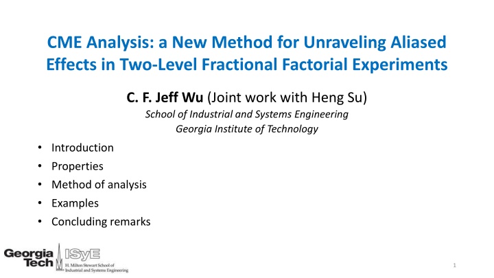
CME Analysis: a New Method for Unraveling Aliased Effects in Two-Level Fractional Factorial Experiments C. F. Jeff Wu (Joint work with Heng Su) School of Industrial and Systems Engineering Georgia Institute of Technology Introduction Properties Method of analysis Examples Concluding remarks 1
Introduction Ever since the founding work by D. J. Finney It has been widely known and accepted that aliased effects in two- level regular designs cannot be de-aliased without adding more runs The following was shown in Wu (2011, Fisher Lecture; 2015 JASA to appear): By using a new framework based on the conditional main effect (CME) the aliasing problems can sometimes be resolved 2
What is a conditional main effect (cme) Consider two factors A and B, each at two levels denoted by + and Main effect of A: ?? ? = ? ? + ? ? . ?? ? =1 2 ? ? + |? + + ? ? + ? Two-factor interaction of A and B: ??? ?,? =1 2 ? ? + |? + ? ? ? Conditional main effect of A given B at +: ??? ? ? + = ? ? + ? + ?(? |?+). (3) Conditional main effect of A given B at -: ??? ? ? = ? ? + ? ?(? |? ). (4) By adding (1) and (2), we have ?? ? + ??? ?,? = ???(?|?+). By subtracting (2) from (1), we have ?? ? ??? ?,? = ???(?|? ). 1 (1) 2 ? ? |? + + ? ? ? . 1 2 ? ? + |? ? ? ? + . (2) 3
Similar property for the design Use short hand notation (A|B+) and (A|B-) instead of cme(A|B+) and cme(A|B-) A|B+ A|B- A|B- A|B+ A A B AB AB Construction definition of cme: ? ? + =1 ? ? =1 + 0 0 + + + + + + 2? + ?? 0 + + 0 + + - - - - 0 0 - - - + - - 2(? ??) 0 0 - - - - - + + /2 From the above relations, it is seen that a cme is related to a main effect and an interaction. Take (A|B+) for example, we call A its parent effect, AB its interaction effect, B its conditioning effect and + its conditioning level 4
Orthogonal modeling For a 2? ? design with k factors, the set of candidate effects consists of 4 ? 2 ? main effects ? 2 Without any restriction, it is hard to find a good model from such a large candidate set. In this work, we restrict the model search to orthogonal models, i.e., effects in a candidate model are orthogonal to each other. cme s 2fi s 5
Orthogonality relations In this work, we restrict the orthogonality to the following notion: Two effects are orthogonal if their inner product is zero Orthogonality relations between cme s and traditional effects cme s are orthogonal to all the traditional effects except for their parent effects and interaction effects. 6
Grouping of cmes and properties 4 1design with I=ABCD Consider a 2?? A + + + + - - - - B + + - - + + - - C + - + - + - + - D + - - + - + + - We categorize cme s into different groups based on their orthogonality relations. 7
Twins cme s having the same parent effect and interaction effect are twins Twin cme s are orthogonal to each other. The 2d space of twin cme s is the same as the 2d space of their parent and interaction effect. Only one of the twin cme s can be chosen. Recall that we have ??? ? ? + = ?? ? + ??? ?,? ???(?|? ) = ?? ? ??? ?,? We can replace a main effect, say A, and a 2fi involving A, say AK, by one of the twin cme s. We refer to A as AK s parental main effect 8
Rule 1 Substitute a pair of 2fi and its parental main effect with similar magnitude with one of the corresponding twin cme s. If the pair have the same sign ??? ? ? + = ?? ? + ??? ?,? will have larger magnitude than both A and AB Replace A and AB with (A|B+) If the pair have the opposite signs ??? ? ? = ?? ? ??? ?,? will have larger magnitude than both A and AB Replace A and AB with (A|B-) 9
Siblings and family cme s having the same parent effect but different interaction effects are siblings. Siblings are NOT orthogonal cme s having the same or fully aliased interaction effects are said to belong to the same family Non-twin cme s in the family are NOT orthogonal 10
Rule 2 Only one cme among its siblings can be included in the model. Only one cme from a family can be included in the model 11
Other cmes and Rule 3 cme s having different parent effect and interaction effect are orthogonal to each other. Rule 3 cme s with different parent effects and different interaction effects can be included in the same model. 12
CME Analysis Recall that we have three rules Based on the three rules, we propose the CME analysis (i). Use the traditional analysis methods such as ANOVA or half-normal plot, to select significant effects, including aliased pairs of effects. Go to (ii). (ii). Among all the significant effects, use Rule 1 to find a pair of fully aliased 2fi and its parental main effect, and substitute them with an appropriate cme. Use Rules 2 and 3 to guide the search and substitution of other such pairs until they are exhausted. cme s with different parent effects and different interaction effects can be included in the same model. Rule 1: Substitute a pair of 2fi and its parental main effect with similar magnitude with one of the corresponding twin cme s. Rule 2: Only one cme among its siblings can be included in the model. Only one cme from a family can be included in the model. Rule 3: 13
Examples We show three examples to illustrate the CME analysis All examples have designs of Resolution IV All examples have significant interactions from traditional analysis 14
Example 1 (Injection Molding) 6 2 design with 2?? ? = ???? = ???? = ???? Traditional analysis: ?~? + ? + ?? (A|B+) The CME analysis Step (ii) A and AB are both significant Consider (A|B+) or (A|B-) 15
Summary of Example 1 In the traditional analysis, we have: ?~? 2.39 10 9+ ? 5.38 10 5+ ?? 0.022% . ?2= 96.24% In the CME analysis, we have: ?~? 6.06 10 10+ ? ? + The second model is more parsimonious and better than the first in terms of p values for significant effects. Two models have comparable ?2values. The cme (A|B+) has a good engineering interpretation: at high screw speed, pressure has a significant effect on shrinkage but not at low speed. 1.72 10 6. ?2= 96.14% 16
Example 2 (Filtration) 4 1 design with ? = ???? 2?? Traditional analysis: ?~? + ?? + ?? + ? + ? (A|D+) The CME analysis (D|B-) Step (ii) A and AD are both significant Consider either (A|D+) or (A|D-) D and DB(=AC) are both significant Consider either (D|B+) or (D|B-) 17
Summary of Example 2 In the traditional analysis, we have: ?~? 0.45% + ?? 0.45% + ?? 0.47% + ? 0.59% + ? 0.82% . ?2= 99.79% In the CME analysis, we have: ?~ ? ? + 0.013% + ?? 0.039% + ? 0.055% + ? 0.089% . ?2= 99.79% ?~ ? ? + 1.96 10 5+ ? ? The third model is the most parsimonious and best in terms of p values for significant effects. All three models have comparable ?2 values. The cme s (A|D+) and (D|B-) in the last two models have good engineering interpretations. 2.72 10 5+ ? 0.026% . ?2= 99.66% 18
Example 3 (Aluminum) 6 2 design with 2?? ? = ???? = ???? = ???? Traditional analysis: ?~? + ? + ?? + ? + ?? Step (ii) E and EB(=AC) are both significant Consider either (E|B+) or (E|B-) F and AF are both significant Consider either (F|A+) or (F|A-) E and ED(=AF) are also a possible pair However (E|D+) and (E|D-) are siblings of (E|B-) The CME analysis (E|B+) (F|A+) 19
Summary of Example 3 In the traditional analysis, we have: ?~? + ? + ? + ?? + ??. (?2= 96.45%) In the CME analysis, we have: ?~ ? ? + + ? + ? + ??. (?2= 94.93%) ?~ ? ? + + ? + ? ? + .(?2= 92.22%) By comparing the ?2 values and p values for significant terms, the third model is not the best. But models 2 and 3 have fewer terms. The cme s (E|B+) and (F|A+) in the last two models have good engineering interpretations, while the 2fi s AC(=BD) and AF(=DE) are aliased. The last two models can be presented to the engineers as alternative choices to the first model. 20
Concluding remarks and future research In this work, we have Proposed the CME analysis to de-alias aliased effects in traditional analysis. Explored the orthogonality relations between cme s and traditional effects. Used three examples to illustrate the advantages of the CME strategy. Future research: Minimum aberration designs for cme analysis (Mukerjee-Wu-Chang, 2015). Using indicator function theory (Sabbaghi 2015) to study aliasing relations. Need to extend to 3? ?designs? Ans. No. (Wu-Hamada 2009 book can handle estimation of interactions for resolution IV 3-level designs.) CME s provide a class of new basis functions in variable selection, new work. Potential impact of CME outside physical experiments, e.g., in medical and social experiments. 21
