Urban Transportation System Modeling

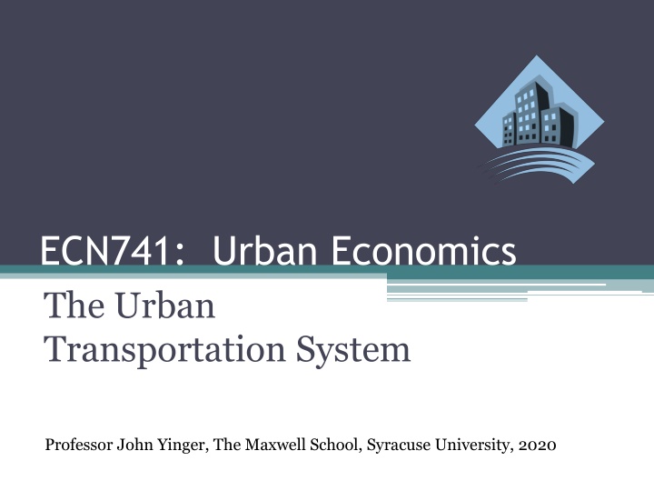
ECN741: Urban Economics The Urban Transportation System Professor John Yinger, The Maxwell School, Syracuse University, 2020

The Urban Transportation System Class Outline 1. Models with street grids 2. Models with street grids and arteries 3. Other models 4. Introduction to traffic congestion

The Urban Transportation System Class Outline 1. Models with street grids 2. Models with street grids and arteries 3. Other models 4. Introduction to traffic congestion

The Urban Transportation System Street Grids The assumption that streets are rays coming out from the center can easily be replaced by the assumption that there is a street grid. This point was made in Alonso, who presents the intuition and examples of iso-cost lines with a grid but does not introduce a grid into a formal urban model. The trick (Yinger, JUE, May 1993) is to use the assumption of an infinitely dense grid to make the math work and to approximate a discrete set of vertical and horizontal streets.

The Urban Transportation System

The Urban Transportation System Alonso Version of Simple Grid

The Urban Transportation System Modeling a Simple Grid In this set-up people travel to work along horizontal and vertical streets. The continuous math literally means that the distance from their house to the nearest street is ignored. In the simplest case, transportation costs equal cost per mile multiplied by Manhattan distance. ( t x = ) + y

The Urban Transportation System Modeling a Simple Grid, 2 In the positive quadrant, this set-up implies that ( T t x y = + T t ) or = y x An iso-cost line is the set of points with equal transportation cost. The above figures imply that y = u, so T = tu and an iso- cost line is defined by y u = x

The Urban Transportation System Modeling a Simple Grid, 4 This equation defines a square iso-cost line; the x- intercept is also at u. Thus the iso-cost line in the positive quadrant is the hypotenuse of right triangle and its length, which is of land supply or L{u}, is = + = = 2 2 2 2 2 d u u u u ( ) L u = = 4 4 2 d u

The Urban Transportation System Modeling a Simple Grid, 5 Recall that when we solved a basic urban model, we assumed that L{u} = 2 u. So all we have done is replace 2 with 4 2. The only thing we have changed is the land constant. All the equations and comparative static results still hold!

The Urban Transportation System Modeling a Simple Grid, 6 But we have substantially altered the geography and characteristics of the urban area. Because population equals the land constant multiplied by an expression, say N*, unaffected by this land constant, we can compare the populations in a radial city and a grid city. 2 4 2 GRID N * N N N = = 1.111 RADIAL * A radial city has 11.1% more people.

The Urban Transportation System Modeling a Simple Grid, 7 We can also compare the physical size of the two cities by comparing the area inside the iso-cost lines that go through . u = 2 Area Area u u = = 1.571 RADIAL 2 2 2 GRID A radial city has 57.1% greater area than a grid city.

The Urban Transportation System Modeling a Simple Grid, 8 Putting these two results together, we can also compare population densities in the two cities. Density equals population divided by area, so . 2 / 4 2 / 2 GRID D N u * 2 2 1 1 RADIAL D N u = = = = = 0.7071 1.4142 * 2 4 2 / 2 2 A radial city has 29.3 percent fewer people per square mile than does a grid city.

The Urban Transportation System Implications for Empirical Work d2 A d3 d1

The Urban Transportation System Implications for Empirical Work From point A radial distance to the CBD = d1 = u, And distance along the grid is ( d + = ) (2 ) 2 d d u 2 3 2 Thus, if the street network is actually like a grid and the empirical work uses radial distance to the CBD, distance measures are too small by as much as 29.3%! measured true 1 d d u = = = = 0.707 1 2 2 2 u 2

The Urban Transportation System Varying Transportation Costs The next step is to allow transportation costs to vary on the vertical and horizontal streets. T t x = + t y h v So in the positive quadrant T t x t = = ;slope h h y t t v v

The Urban Transportation System Varying Transportation Costs, 2 Note that in this figure, d th < tv and the city shape stretches in the low-cost direction.

The Urban Transportation System Varying Transportation Costs, 3 Now anchoring an iso-cost on the vertical axis, we have T t u = = t x t y + v h t t v = h y u x v The iso-cost line runs from (0,u) to ((tv/th)u, 0).

The Urban Transportation System Varying Transportation Costs, 4 So the length of an is-cost line is: 2 2 t t t t = + = + 2 1 v v d u u u h h And the land constant is 2 t t = + 4 4 1 v d h

The Urban Transportation System Varying Transportation Costs, 5 Recall that the population of a radial city is 11.1% larger than the population of a grid city with the same t. How much lower would thhave to be for a stretched grid city to have the same population as the radial city? The two land constants, and hence the two populations are the same if 2 t = + 2 4 1 t h 2 t = = 1 1.211 2 t h

The Urban Transportation System Varying Transportation Costs, 6 It follows that th would have to equal t divided by 1.211, which is the same as saying that th would have to 17.42% smaller than t. ( 1-(1/1.211) = 1- 0.8258 = .1742) In other words, a grid city s disadvantage in using space caused by its longer commuting distances can be offset by lowering travel costs in one direction by 17.42%. As an exercise: Show that if N is equal in the two cities, the radial city s land area is greater by 29.8%.

The Urban Transportation System Questions Why is the map of a city different with a grid than with radial highways? How can modeling of the transportation network improve estimation of the housing price gradient?

The Urban Transportation System Class Outline 1. Models with street grids 2. Models with street grids and arteries 3. Other models 4. Introduction to traffic congestion

The Urban Transportation System Grids Plus Arteries The next step in the analysis is to add commuting arteries, which could be freeways, subways, or trains. The analysis depends on the relationship between the arteries and the grid. The two simplest cases are in the following graphs.

The Urban Transportation System Grids Plus Arteries, 2

The Urban Transportation System Alonso Version of Grid with Arteries

The Urban Transportation System Commuting Sheds The introduction of grids adds a key new concept, namely a commuting shed. A commuting shed is analogous to a water shed; People on one side of a boundary commute in one direction, whereas people on the other side commute the other way Just like water that falls on one side of the Continental Divide flows to the Pacific Ocean, whereas water that falls on the other side flows to the Atlantic Ocean.

The Urban Transportation System Commuting Sheds, 2 Shed boundaries Commuting paths Artery

The Urban Transportation System Vertical and Horizontal Arteries This shed picture describes vertical and horizontal arteries. The shed boundary is defined by t y + = + t x t x t y a h a v In the positive quadrant, this is t t t t = a h y x a v

The Urban Transportation System Vertical and Horizontal Arteries, 2 The iso-cost is defined by = T t y t x a h or t t T t = h y x a a

The Urban Transportation System Vertical and Horizontal Arteries, 3 As before, define T = tau; the iso-cost becomes t u y t t x t t = = a h h u x a a The slope is less than (-1) because th > ta.

The Urban Transportation System Vertical and Horizontal Arteries, 4 Iso-Cost Line (0,u) d Point that is on shed and iso- cost line =(x*,y*) City stretches out along arteries.

The Urban Transportation System Vertical and Horizontal Arteries, 5 Pooling earlier results for shed and iso-cost: t y x t t t t t = = a h h u x a v a Solving for (x*,y*) ( ) ( ) t t t t t t = = * and * a a v a a h x u y u 2 2 ( ) a t ( ) a t h v t t h v t t

The Urban Transportation System Vertical and Horizontal Arteries, 6 Finally, plugging both points into the standard distance formula, we find that 2 2 ( ) ( ) t t t t t t = + 2 2 1 a a v a a h d u u 2 2 ( ) a t ( ) a t h v t t h v t t + 2 2 2 (( ) t ( ) )( v t ) t t = a a v u 2 2 (( ) t ) h v t t a

The Urban Transportation System Vertical and Horizontal Arteries, 7 Once again, we find that extending the transportation system does not change the algebra of the basic model, although it does change the map. If tv = th, the new land constant is simply 8d, and all the equations and comparative statics from the basic model still hold. If tv th , then the formula for the length of the iso-cost line below the artery switches the tvand th terms and the length is 4 times the sum of the two lengths.

The Urban Transportation System Diagonal Arteries The next case to consider is diagonal arteries. We will keep it simple, with the same costs on vertical and horizontal streets = tg And with arteries at a 45 degree angle to the grid. This set-up is similar to the core design of Washington, D.C., with the Capitol as the CBD and the Mall as one of the arteries.

The Urban Transportation System Diagonal Arteries, 2 (0,u) Artery d y - x x 2 Shed Boundary

The Urban Transportation System Diagonal Arteries, 3 Thus, the equation for an iso-cost line is = = + ( ) 2 T t u t y x t x g g a or t t = + 1 2 a y u x g

The Urban Transportation System Diagonal Arteries, 4 Note that the slope of the iso-cost line in the positive quadrant could be positive as drawn, yielding a star shape, or negative, yielding a hexagon. The hexagon case arises if: t t 1 2 0 or 2 a t t g a g

The Urban Transportation System Diagonal Arteries, 5 Because y = x on the artery, we can write t g = = x y u 2 t a This gives us the coordinates of the point on the artery, and we can solve for the distance. 2 t t t t g g = + { } 8 L u 1 2 u a a

The Urban Transportation System Diagonal Arteries, 6 Diagonal arteries do not have to be at a 45 degree angle, of course. Yinger (JUE, May 1993) also shows how to find the land constant with any number of arteries set at any angles to the grid. Anas-Moses and Baum-Snow also have models with multiple arteries. In some cases, one can have travel in the wrong direction because the savings from getting to the artery faster offset the backwards direction.

The Urban Transportation System Diagonal Arteries, 7 One straightforward way to handle multiple arteries with a grid is to make the arteries evenly spaced, add a grid that is perpendicular to each artery, and allow this grid to rotate at each commuting shed boundary. This set-up keeps the math simple. This is the design in Amsterdam or Palmanova, Italy. A map of Palmanova is on the next slide.

The Urban Transportation System Palmanova, Italy https://historicalmaps.wordpress.com/2015/06/09/map-of-palmanova-italy-ca-1572/

The Urban Transportation System Arteries and Maps As indicated earlier, adding arteries changes the map of an urban area: the area extends farther from the center along a high-speed artery (or, for that matter, along high-speed streets). This impact can be observed in many places, as development extends along main streets or highways. One well-known urban scholar, Nate Baum-Snow, uses a closed urban model to argue that the building of arteries caused suburbanization. (N. Baum-Snow, Did Highways Cause Suburbanization? , QJE, May 2007)

The Urban Transportation System Arteries and Maps, 2 The Baum-Snow work is interesting and well done. But in a theory paper on which his QJE paper draws ( Suburbanization and Transportation in the Monocentric Model, JUE, November 2007), he says: The main innovation of this model is that it incorporates highways into the transportation infrastructure of a monocentric city. Highways are modeled as linear rays emanating from the city s core along which the travel speed is faster than on surface streets. Two earlier articles in the same journal already presented his innovation: Anas-Moses (JUE, April 1979), which he cites, and Yinger (JUE, May 1993), which he does not cite. Make sure you use Google scholar!

The Urban Transportation System Class Outline 1. Models with street grids 2. Models with street grids and arteries 3. Other models 4. Introduction to traffic congestion

The Urban Transportation System Other Forms of High-Speed Modes These methods can be applied to many other types of high-speed modes that do not go to the CBD. This point was clearly recognized by Alonso (whose contributions are also not mentioned by Baum-Snow). The next two slides give one alternative arrangement in Yinger and another from Alonso s book.

The Urban Transportation System City with Several Vertical Arteries

The Urban Transportation System Alonso: Arteries and Square Beltway

The Urban Transportation System Anas-Moses A final type of transportation system to discuss is one devised by Anas and Moses (JUE, April 1979). They assume two modes: circular streets that lead to commuting arteries and a network of local streets that can be approximated by a standard model. They show that people making different mode choices will sort into different locations (or, equivalently, because all people are alike, people who live in different places will make different mode choices).