Use-Case Points for Software Size Estimation
This presentation delves into the use of Use-Case Points for estimating software project size in IT project management, highlighting its importance in effort estimation and requirements engineering processes. Various methods and techniques for software effort estimation are discussed along with insights on use cases and scope management.

Download Presentation

Please find below an Image/Link to download the presentation.
The content on the website is provided AS IS for your information and personal use only. It may not be sold, licensed, or shared on other websites without obtaining consent from the author.If you encounter any issues during the download, it is possible that the publisher has removed the file from their server.
You are allowed to download the files provided on this website for personal or commercial use, subject to the condition that they are used lawfully. All files are the property of their respective owners.
The content on the website is provided AS IS for your information and personal use only. It may not be sold, licensed, or shared on other websites without obtaining consent from the author.
E N D
Presentation Transcript
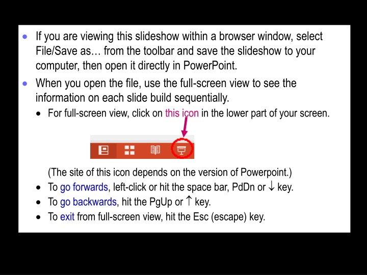
If you are viewing this slideshow within a browser window, select File/Save as from the toolbar and save the slideshow to your computer, then open it directly in PowerPoint. When you open the file, use the full-screen view to see the information on each slide build sequentially. For full-screen view, click on this icon in the lower part of your screen. (The site of this icon depends on the version of Powerpoint.) To go forwards, left-click or hit the space bar, PdDn or key. To go backwards, hit the PgUp or key. To exit from full-screen view, hit the Esc (escape) key.
Sample-size Estimation: Theory and Specific Issues Will G Hopkins Victoria University Melbourne, Australia Background Sample Size for Statistical Significance how it works Sample Size for Clinical Outcomes how it works Sample Size for Suspected Large True Effects how it works Sample Size for Superiority Testing Sample Size for Equivalence Testing Sample Size for Precise Estimates how it works Specific Issues Sample size in other studies; smallest effects; big effects, on the fly, small sample sizes, post-hoc justification; design, drop-outs, clustering; validity and reliability; comparing groups, subgroup comparisons; modifiers; individual differences, mediators; mixing unequal sexes; multiple effects; case series; single subjects; measurement studies, simulation Conclusions View as a slideshow and click on the above topics to link to the slides.
Background We study an effect in a sample, but we want to know about the effect in the population. The larger the sample, the closer we get to the population. Too large is unethical, because it's wasteful. Too small is unethical, because the outcome might be indecisive. And you are less likely to get your study funded and published. The traditional approach is based on statistical significance. But to "retire statistical significance", we need new approaches. I present here the traditional approach, two new approaches for magnitude-based decisions (MBD), an extension of MBD to minimal effects and equivalence testing, and some useful stuff that applies to most approaches. A spreadsheet for these approaches is available at sportsci.org.
Sample Size for Statistical Significance In this old-fashioned approach, you decide whether an effect is real : that is, statistically significant (non-zero). If you get significance and you re wrong, it s a false-positive or Type I statistical error. If you get non-significance and you re wrong, it s a false negative or Type II statistical error. The defaults for acceptably low error rates are 5% and 20%. The false-negative rate is for the smallest important value of the effect, or the minimum clinically important difference . Solve for the sample size by assuming a sampling distribution for the effect.
Sample Size for Statistical Significance: How It Works The Type I error rate (5%) defines a critical value of the statistic. If observed value > critical value, the effect is significant. SIGNIFICANT NON-SIG probability distribution of observed values, if true value = 0 critical value SIGNIFICANT distribution of observed values, if true value = smallest important value area = 20% area = 2.5% smallest important value area = 2.5% negative positive 0 value of effect statistic When true value = smallest important value, the Type II error rate (20%) = chance of observing a non-significant value. Solve for the sample size (via the critical value).
Sample Size for Clinical Outcomes In the first new approach, the decision is about whether to use the effect in a clinical or practical setting. If you decide to use a harmful effect, it s a false-positive or Type 1 clinical error. If you decide not to use a beneficial effect, it s a false-negative or Type 2 clinical error. Suggested defaults for acceptable error rates are 0.5% and 25%. Benefit and harm are defined by the smallest clinically important effects. Solve for the minimum desirable sample size by assuming a sampling distribution. Sample sizes are ~1/3 those for statistical significance. The traditional approach is too conservative? P=0.05 with the traditional sample size implies one chance in about half a million of the effect being harmful.
Sample Size for Clinical Outcomes: How It Works The smallest clinically important effects define harmful, beneficial and trivial values. At some decision value, Type 1 clinical error rate = 0.5%. and Type 2 clinical error rate = 25% HARMFUL TRIVIAL probability distribution of true values if observed value = decision value BENEFICIAL decision value smallest harmful value smallest beneficial value area = 25% area = 0.5% negative positive 0 value of effect statistic Now solve for the minimum desirable sample size (and the decision value).
Sample Size for Suspected Large True Effects The decision value is such that chance of observing a smaller value, given the true value, is the Type 2 error rate (25%) and if you observe the decision value, there has to be a chance of harm equal to the Type 1 error rate (0.5%). HARMFUL TRIVIAL BENEFICIAL distribution of observed values, given the true value probability distribution of true values, when observed value = decision value decision value true value area = 25% smallest harmful value area = 0.5% negative positive 0 value of effect statistic Now solve for the sample size (and the decision value).
Sample Size for Superiority Testing In superiority testing, the researcher wants a high chance of deciding an effect is substantial (+ive, say), when the true effect is a substantial expected value greater than the smallest important. So the calculation for a suspected true large effect applies. But when you do the study, you want this outcome: the chance that the effect is substantially +ive is >95% (very likely). That is, you want the chance that the effect is not substantially +ive to be <5%. You can achieve that by replacing the smallest harmful value with the smallest important +ive value in the calculation for sample size, and by setting the Type-1 and Type-2 error rates to 5%. If the suspected true substantial effect is borderline small- moderate, the sample size is the same as for MBD. So MBD should satisfy the proponents of superiority testing.
Sample Size for Equivalence Testing Equivalence testing is similar to superiority testing, but with a high chance of deciding an effect is trivial, when the true effect is an expected trivial value smaller than the smallest important. So when you do the study, you want this outcome: the chance that the effect is trivial is >95% (very likely). That is, you want <5% chance that the effect is not substantial +ive. In the calculation for sample size, you can achieve that by making the smallest beneficial value the smallest important +ive value, by replacing the smallest harmful value with the expected trivial value, and by setting the Type-1 and Type-2 errors to 5%. If the true trivial effect is half the smallest important, the sample size 16x that for MBD impractical for most researchers. Equivalence testing is an option in a meta-analysis, if the effective sample size is large enough.
Sample Size for Precise Estimates In the new approach, the decision is about whether the effect has adequate precision in a non-clinical setting. Precision is defined by the compatibility interval: the uncertainty in the true effect. The suggested default level of compatibility is 90%. Adequate implies a compatibility interval that does not permit substantial values of the effect in a positive and negative sense. Positive and negative are defined by the smallest important effects. Solve for the minimum desirable sample size by assuming a sampling distribution. Sample sizes are almost identical to those for clinically important effects with Type 1 and 2 error rates of 0.5% and 25%. The Type 1 and 2 error rates are each 5%. There is also the same reduction in sample size for suspected large true effects.
Sample Size for Precise Estimates: How It Works The smallest substantial positive and negative values define ranges of substantial values. Precision is unacceptable if the 90% CI overlaps substantial positive and negative values. SUBSTANTIAL NEGATIVE TRIVIAL unacceptable acceptable acceptable SUBSTANTIAL POSITIVE acceptable worst case smallest substantial negative value smallest substantial positive value negative positive 0 Solve for the sample size in the acceptable worst case. For superiority and equivalence sample sizes, the 90% CI also just fits between the values required for the smallest substantials.
Specific Issues Check your assumptions and sample-size estimate by comparing with those in published studies. But be skeptical about the justifications you see in the Methods. Most authors either do not mention the smallest important effect, choose a large one to make the sample size acceptable, or make some other serious mistake with the calculation. You can justify a sample size on the grounds that it is similar to those in similar studies that produced clear outcomes. But effects are clear often because they are substantial. If yours turns out to be smaller, you may need a larger sample. For a crossover or controlled trial, you can use the sample size, value of the effect, and p value or compatibility limits in a similar published study to estimate sample size in your study. See the sample-size spreadsheet for more.
Sample size is sensitive to the value of the smallest effect. Halving the smallest effect quadruples the sample size. You have to justify your choice of smallest effect. Difference or change in means: the value associated with a smallest important difference or change in health, wealth or competitive performance. Failing that, Cohen's d of 0.20: a standardized difference or change in the mean of 0.20 of the appropriate between-subject SD. Standardization also works for psychometrics derived from multi-item inventories and for team-sport fitness tests and performance indicators. Single Likert or visual-analog scales: 10% of "full-scale deflection". Correlation: 0.10 Proportion, hazard or count ratio: 0.9 for a decrease, 1/0.9 = 1.11 for an increase. Proportion difference for matches won or lost in close games: 10%. Change in competitive performance score of a top athlete: 0.3 of the within-athlete variability between competitions. Big mistakes occur here!
Bigger effects need smaller samples for decisive outcomes. So start with a smallish cohort, then add more if outcome is unclear. Aka group-sequential design , or sample size on the fly . Estimate sample size of a second cohort using the effect in the first cohort as a suspected large effect. There could be small but unknown upward bias in effect magnitude. An unavoidablysmallsample size is ethically defensible if the true effect is large enough for the outcome to be conclusive. And if it turns out inconclusive, argue that it will still set useful limits on the likely magnitude of the effect and should be published, so it can contribute to a meta-analysis. Provide a "post hoc" justification of sample size: the size if you were to use a second cohort, and the minimum desirable. Even minimum desirable sample sizes can produce inconclusive outcomes, thanks to sampling variation. The risk of such an outcome, estimated by simulation, is at most ~10%. Eliminate by increasing sample size by up to 25%.
Sample size depends on the design. Non-repeated measures studies (cross-sectional, prospective, case-control) usually need hundreds or thousands of subjects. Repeated-measures studies (controlled trials and crossovers) usually need scores or hundreds of subjects. Post-only crossovers need less than parallel-group controlled trials (down to ), provided subjects are stable during the washout. Sample-size estimates for prospective studies and controlled trials should be inflated by 10-30% to allow for drop-outs depending on the demands placed on the subjects, the duration of the study, and incentives for compliance. When subjects within clusters (e.g., players within several teams) tend to have similar effects, the effective sample size is less than the total number of subjects. But it's difficult to estimate what the sample size should be. So you might have to do sample size "on the fly".
Sample size depends on validity and reliability. Effect of validity of a dependent or predictor variable: Sample size is proportional to 1/v2 = 1+e2/SD2, where v is the validity correlation of the dependent variable, e is the error of the estimate, and SD is the between-subject standard deviation of the criterion variable in the validity study. So v = 0.7 implies twice as many subjects as for r = 1. Effect of reliability of a repeated-measures dependent variable: Sample size is proportional to (1 r) = e2/SD2, where r is the test-retest reliability correlation coefficient, e is the error of measurement, and SD is the observed between-subject standard deviation. So really small sample sizes are possible with high r or low e. But avoid <10 in any group, because such small samples can easily misrepresent the population.
Make any compared groups equal in size for smallest total sample size. If the size of one group is limited by availability of subjects, recruit more subjects for the comparison group. But >5x more gives no practical increase in precision. Example: 100 cases plus 10,000 controls is little better than 100 cases plus 500 controls. Both are equivalent to 200 cases plus 200 controls. With designs involving comparison of effects in subgroups Assuming equal numbers in two subgroups, you need twice as many subjects to estimate the effect in each subgroup separately. But you need twice as many again to compare the effects. Example: a controlled trial that would give adequate precision with 20 subjects would need 40 females and 40 males for comparison of the effect between females and males. So don't go there as a primary aim without adequate resources.
Quadrupling sample size for subgroup analyses applies also to estimating thelinear modifying effect of a continuous predictor. You evaluate the effect of 2 SD of the predictor. You are effectively comparing the effect in two groups of subjects: a group 1 SD above the mean and a group 1 SD below the mean. Adjustment of an effect to the mean value of a moderator can actually reduce the sample size required for the effect itself. If the moderator has a substantial effect, it explains otherwise unexplained variance. The most important example is adjustment to the mean value of the dependent variable at baseline in a crossover or controlled trial. The reduction in sample size depends on the relative magnitudes of the within- and between-subject SDs. You should adjust for this and other potential moderators, even if their effects are unclear.
Individual differences and responses are due to modifying effects of subject characteristics. So you need 4x as many subjects to account for them with linear predictors. This bigger sample may not give adequate precision for the standard deviation representing individual responses to a treatment. Required sample size in the worst-case scenario of zero mean change and zero individual responses is impractically large: 6.5n2, where n is the sample size for adequate precision of the mean! A potential mediator of a treatment effectin a crossover or controlled trial is analyzed by including its change score as a main-effect predictor in the linear model. The required sample size is twice that for the mean effect. But to allow for a different mechanism in control and experimental groups, include the mediator as an interaction with the group effect. The required sample size is then 4x that for the mean effect.
Mixing unequal numbers of females and males (or other different subgroups) in a small study is not a good idea. You are supposed to analyze the data by assuming there could be a difference between the subgroups. The effect under study is effectively estimated separately in females and males, then averaged. Here is an example of the resulting effective sample size (for 90% compatibility limits): No. of males 10 10 10 10 No. of females 10 5 4 3 Total Effective sample size 20 13 10 7 sample size 20 15 14 13 Less than the number of males! So, if you include a smaller sample size of the other gender, analyze the genders separately. Compare the genders with a third analysis, but the comparison may be unclear.
With more than one effect, you need a bigger sample size to constrain the overall chance of error. For example, suppose you got chances of harm and benefit for Effect #1: 0.4% and 72% for Effect #2: 0.3% and 56%. If you use both, chances of harm = 0.7% (> the 0.5% limit). But if you don t use #2 (say), you fail to use an effect with a good chance of benefit (> the 25% limit). Solution: increase the sample size to keep total chance of harm <0.5% for effects you use, and total chance of benefit <25% for effects you don t use. For n independent effects, set the Type 1 error rate (%) to 0.5/n and the Type 2 error rate to 25/n. The spreadsheet shows you need 50% more subjects for n=2 and more than twice as many for n=5. For interdependent effects there is no simple formula.
Sample size for a case series defines norms adequately, via the mean and SD of a given measure. The default smallest difference in the mean is 0.2 SD, so the uncertainty (90% compatibility interval) needs to be <0.2 SD. Resulting sample size is that of a cross-sectional study, ~70. Resulting uncertainty in the SD is 1.15, which is OK. Smaller sample sizes will lead to less confident characterization of future cases. Larger sample sizes are needed to characterize percentiles, especially for non-normally distributed measures.
For single-subject studies, sample size is the number of repeated observations on the single subject. Use the sections of the sample-size spreadsheet for cross- sectional studies. Use the value for the smallest important difference that applies to sample-based studies. What matters for a single subject is the same as what matters for subjects in general. Use the subject s within-subject SD as the between-subject SD . The within is often << the between, so sample size is often less than for a cross-sectional study (but still larger than you would like). Assume any trend-related autocorrelation will be accounted for by your model and will therefore not entail a bigger sample. But estimating the number of measurements to quantify a trend is too difficult with an equation. Instead use simulation, available in a spreadsheet in the workbook for monitoring individuals.
Sample size for measurement studies is not included in available software for estimating sample size. Very high reliability and validity can be characterized with as few as 10 subjects. More modest validity and reliability (correlations ~0.7-0.9; errors ~2-3 the smallest important effect) need samples of 50-100 subjects. Studies of factor structure need many hundreds of subjects. See the article and slideshow on validity and reliability for more. Try simulation to estimate sample size for complex designs. Make reasonable assumptions about errors and relationships between the variables. Generate data sets of various sizes using appropriately transformed random numbers. Analyze the data sets to determine the sample size that gives acceptable width of the compatibility interval.
Conclusions You can base sample size on acceptable rates of clinical errors or adequate precision. Both make more sense than sample size based on statistical significance and both lead to smaller samples. These methods are innovative and not yet widely accepted. So I recommend using superiority testing in addition to, or instead of, the new approaches. Avoid NHST sample-size estimation, as we are supposed to "retire statistical significance". Remember to increase sample size for measures with low validity, multiple effects, comparison of subgroups, moderators, mediators, and individual differences or responses. If your sample size is limited to tens of subjects, try to do an intervention (preferably as a crossover) with a reliable dependent variable.
Presentation, article and spreadsheets: See Sportscience 24, 17-27, 2020